1 Introduction
Image registration is the problem of aligning images into a common coordinate system such that the discrete pixel locations have the same semantic information. It is a common pre-processing step for many applications, e.g. the statistical analysis of imaging data and computer-aided diagnosis through comparison with an atlas. Image registration methods based on deep learning tend to incorporate task-specific knowledge from large datasets, whereas traditional methods are more general purpose. Many established models are based on the iterative optimisation of an energy function consisting of task-specific similarity and regularisation terms, which has to be done independently for every pair of images in order to calculate the deformation field (Schnabel et al., 2001; Klein et al., 2009; Avants et al., 2014).
DLIR (de Vos et al., 2019) and VoxelMorph (Balakrishnan et al., 2018, 2019; Dalca et al., 2018, 2019) changed this paradigm by learning a function that maps a pair of input images to a deformation field. This gives a speed-up of several orders of magnitude at inference time and maintains an accuracy comparable to traditional methods. An overview of state-of-the-art models for image registration based on deep learning can be found in Lee et al. (2019).
Due to the perceived conceptual difficulty and computational overhead, Bayesian methods tend to be shunned when designing medical image analysis algorithms. However, in order to fully explore the parameter space and lessen the impact of ad-hoc hyperparameter choices, it is desirable to use Bayesian models. In addition, with help of open-source libraries with automatic differentiation like PyTorch, the implementation of even complex Bayesian models for image registration is very similar to that of non-probabilistic models.
In this paper, we make use of the stochastic gradient Markov chain Monte Carlo (SG-MCMC)algorithm to design an efficient posterior sampling algorithm for 3D non-rigid image registration. SG-MCMCis based on the idea of stochastic gradient descent interpreted as a stochastic process with a stationary distribution centred on the optimum and whose covariance can be used to approximate the posterior distribution (Chen et al., 2016; Mandt et al., 2017). SG-MCMCmethods have been useful for training generative models on very large datasets ubiquitous in computer vision, e.g. Du and Mordatch (2019); Nijkamp et al. (2019); Zhang et al. (2020). We show that they are also applicable to image registration.
This work is an extended version of Grzech et al. (2020), where we first proposed use of the SG-MCMCalgorithm for non-rigid image registration. The code to reproduce the results is available in a public repository: https://github.com/dgrzech/ir-sgmcmc. The following is a summary of the main contributions of the previous work:
- 1.
We proposed a computationally efficient SG-MCMCalgorithm for three-dimensional diffeomorphic non-rigid image registration;
- 2.
We introduced a new regularisation loss, which allows to carry out inference of the regularisation strength when using a transformation parametrisation with a large number of degrees of freedom;
- 3.
We evaluated the model both qualitatively and quantitatively by analysing the output transformations, image registration accuracy, and uncertainty estimates on inter-subject brain magnetic resonance imaging (MRI)data from the UK Biobank dataset.
In this version, we extend the previous work:
- –
We provide more details on the Bayesian formulation, including a comprehensive analysis of the learnable regularisation loss, as well as a more in-depth analysis of the model hyperparameters and hyperpriors;
- –
We conduct additional experiments in order to compare the uncertainty estimates output by variational inference (VI), SG-MCMC, and VoxelMorph qualitatively, as well as quantitatively by analysing the Pearson correlation coefficient between the displacement and label uncertainties;
- –
We analyse the differences between uncertainty estimates when the SG-MCMCalgorithm is initialised to different transformations and when using different parametrisations of the transformation, including non-parametric stationary velocity fields (SVFs)and SVFsbased on B-splines; and
- –
We include a detailed evaluation of the computational speed and of the output transformation smoothness.
2 Related work
The problem of uncertainty quantification in non-rigid image registration is controversial because of ambiguity regarding the definition of uncertainty as well as the accuracy of uncertainty estimates (Luo et al., 2019). Uncertainty quantification in probabilistic image registration relies either on variational Bayesian methods (Simpson et al., 2012, 2013; Wassermann et al., 2014), which are fast and approximate, and popular within models based on deep learning (Dalca et al., 2018; Liu et al., 2019; Schultz et al., 2019), or Markov chain Monte Carlo (MCMC)methods, which are slower but enable asymptotically exact sampling from the posterior distribution of the transformation parameters. The latter include e.g. Metropolis-Hastings used for intra-subject registration of brain MRIscans (Risholm et al., 2010, 2013) and estimating delivery dose in radiotherapy (Risholm et al., 2011), reversible-jump MCMCused for cardiac MRI(Le Folgoc et al., 2017), and Hamiltonian Monte Carlo used for atlas building (Zhang et al., 2013).
Uncertainty quantification for image registration has also been done via kernel regression (Zöllei et al., 2007; Janoos et al., 2012) and deep learning (Dalca et al., 2018; Krebs et al., 2019; Heinrich, 2019; Sedghi et al., 2019). More generally, Bayesian frameworks have been used e.g. to characterize image intensities (Hachama et al., 2012) and anatomic variability (Zhang and Fletcher, 2014).
One of the main obstacles to a more widespread use of MCMCmethods for uncertainty quantification is the computational cost. This was recently tackled by embedding MCMCin a multilevel framework (Schultz et al., 2018). SG-MCMCwas previously used for rigid image registration (Karabulut et al., 2017). It has also been employed in the context of unsupervised non-rigid image registration based on deep learning, where it allowed to sample from the posterior distribution of the network weights, rather than directly the transformation parameters (Khawaled and Freiman, 2020).
Previous work on data-driven regularisation focuses on transformation parametrisations with a relatively low number of degrees of freedom, e.g. B-splines (Simpson et al., 2012) and a sparse parametrisation based on Gaussian radial basis functions (RBFs)(Le Folgoc et al., 2017). Limited work exists also on spatially-varying regularisation, again with B-splines (Simpson et al., 2015). Deep learning has been used for spatially-varying regularisation learnt using more than one image pair (Niethammer et al., 2019). Shen et al. (2019) introduced a related model which could be used for learning regularisation strength based on a single image pair but suffered from non-diffeomorphic output transformations and slow speed.
3 Registration model
We denote an image pair by , where and are a fixed and a moving image respectively. The goal of image registration is to align the underlying domains and with a transformation , i.e. to calculate parameters such that . The transformation is often expected to possess desirable properties, e.g. diffeomorphic transformations are smooth and invertible, with a smooth inverse.
We parametrise the transformation using the SVFformulation (Arsigny et al., 2006; Ashburner, 2007), which we briefly review below. The ordinary differential equation (ODE)that defines the evolution of the transformation is given by:
| (1) |
where is the identity transformation and . If the velocity field is spatially smooth, then the solution to Equation 1 is a diffeomorphic transformation. Numerical integration is done by scaling and squaring, which uses the following recurrence relation with steps (Arsigny et al., 2006):
| (2) |
The Bayesian image registration framework that we present is not limited to SVFs. Moreover, there is a very limited amount of research on the impact of the transformation parametrisation on uncertainty quantification. Previous work on uncertainty quantification in image registration characterised uncertainty using a single transformation parametrisation, e.g. a small deformation model using B-splines in Simpson et al. (2012), the finite element (FE)method in Risholm et al. (2013), and multi-scale Gaussian RBFsin Le Folgoc et al. (2017), or a large deformation diffeomorphic metric mapping (LDDMM)in Wassermann et al. (2014).
To help understand the potential impact of the transformation parametrisation on uncertainty quantification, we also implement SVFsbased on cubic B-splines (Modat et al., 2012). In this case, the SVFconsists of a grid of B-spline control points, with regular spacing voxel. The dense SVFat each point is a weighted combination of cubic B-spline basis functions (Rueckert et al., 1999). To calculate the transformation based on the dense velocity field, we again use the scaling and squaring algorithm in Equation 2.
3.1 Likelihood model
The likelihood specifies the relationship between the data and the transformation parameters by means of a similarity metric. In probabilistic image registration, it usually takes the form of a Boltzmann distribution (Ashburner, 2007):
| (3) |
where is the similarity metric and an optional set of hyperparameters.
Local cross-correlation (LCC), which is invariant to linear intensity scaling, is a popular similarity metric but not meaningful in a probabilistic context. For this reason, instead of the sum of the voxel-wise product of intensities, like in standard LCC, we opt for the sum of voxel-wise squared differences of images standardised to zero mean and unit variance inside a local neighbourhood of five voxels. This way, we can benefit from robustness under linear intensity transformations, as well as desirable properties of a Gaussian mixture model (GMM)of intensity residuals, i.e. robustness to outlier values caused by acquisition artefacts and misalignment over the course of registration (Le Folgoc et al., 2017).
Let and be respectively the fixed and the warped moving image with intensities standardised to zero mean and unit variance inside a neighbourhood of five voxels. For each voxel, the intensity residual , , is assigned to the -th component of the mixture, , if the categorical variable is equal to , in which case it follows a normal distribution 111In order to reduce the notation clutter we omitted the voxel index for the fixed and moving images.. The component assignment follows a categorical distribution and takes value with probability . We use the same GMMof intensity residuals on a global basis rather than per neighbourhood. In all experiments it has components, which we determine to be sufficient for a good model fit.
We also use the scalar virtual decimation factor to account for the fact that voxel-wise residuals are not independent. This prevents over-emphasis on the data term and allows to better calibrate uncertainty estimates (Groves et al., 2011; Simpson et al., 2012). The full expression of the image similarity term is given by:
| (4) |
3.2 Transformation priors
In Bayesian models, the transformation parameters are typically regularised with use of a multivariate normal prior that ensures smoothness:
| (5) |
where is a scalar parameter that controls the regularisation strength, and is the matrix of a differential operator. Here we assume that represents the gradient operator, which penalises the magnitude of the 1 derivative of a velocity field. Note that .
The regularisation weight can either be fixed or estimated from data. The latter has been done successfully only for transformation parametrisations with a relatively low number of degrees of freedom, e.g. B-splines (Simpson et al., 2012) and a sparse parametrisation (Le Folgoc et al., 2017). In case of an SVF, where the number of degrees of freedom is orders of magnitude higher, the problem is more difficult. However, a reliable method to adjust regularisation strength based on data is crucial, as both the output transformation and registration uncertainty are highly sensitive to regularisation. In order to infer the regularisation strength, we specify a log-normal prior on the scalar regularisation energy , and derive a prior on the underlying SVF:
| (6) | ||||
| (7) |
where is the number of degrees of freedom, i.e. the count of transformation parameters in all three directions. Given (semi-)informative hyperpriors on and , which we discuss in the next section, we can adjust the regularisation strength to the input images. The full expression of the regularisation term is given by:
| (8) |
It is worth noting that the traditional regularisation with a fixed regularisation weight in Equation 5 actually belongs to this family of regularisation losses. If we specify a gamma prior instead of a log-normal prior on the scalar regularisation energy , we get:
| (9) | ||||||
| (10) | ||||||
| (11) |
3.3 Hyperpriors
We set the likelihood GMMhyperpriors similarly to Le Folgoc et al. (2017), with the mixture precision parameters assigned independent log-normal priors and the mixture proportions with an uninformative Dirichlet prior , where .
Regularisation parameters require informative priors due to the difficulty of learning the regularisation strength based on a single image pair. Because of a gamma prior on the regularisation energy , we can rely on the familiar regularisation weight to initialise the logarithm of the regularisation energy to the expected value of the logarithm of the gamma distribution, i.e. , where is the digamma function. The value of this expression is sharply peaked if the number of degrees of freedom is large, which yields a very informative prior on . More details on how to calculate the expected value of the logarithm of a gamma distribution can be found in Section A.
The choice of a hyperprior on the scale parameter , which controls the amount of deviation of from the location parameter , is more intuitive. Here we use a log-normal prior .
4 Variational inference
Image registration methods often rely on VIfor uncertainty quantification. We only use VIto initialise the SG-MCMCalgorithm, which also lets us compare the uncertainty estimates output by approximate and asymptotically exact methods for sampling from the posterior distribution of transformation parameters.
We assume that the posterior distribution is a multivariate normal distribution . To find parameters and , we maximise the evidence lower bound (ELBO)(Jordan et al., 1999):
| (12) |
where is the Kullback-Leibler divergence (KL-divergence)between the approximate posterior and the prior . Like in traditional image registration, the energy function consists of the sum of similarity and regularisation terms, with an additional term for the entropy of the posterior distribution . We show how to calculate this term in Section B.
It is not possible to calculate every element of the covariance matrix due to high dimensionality of the problem. Instead, we approximate the covariance matrix as a sum of diagonal and low-rank parts, i.e. , with and , where is a hyperparameter which determines the parametrisation rank. Using a multivariate normal distribution as the approximate posterior distribution of transformation parameters is common in probabilistic image registration. The key difference in our work is the diagonal + low-rank parametrisation of the covariance matrix. Most recent image registration models with an SVFtransformation parametrisation are based on deep learning and make the assumption of a diagonal covariance matrix (Dalca et al., 2018; Krebs et al., 2019).
We use the reparametrisation trick with two samples per update to backpropagate with respect to the variational posterior parameters:
| (13) | ||||
In order to make the optimisation less susceptible to undesired local maxima of the ELBO, we take advantage of Sobolev gradients (Neuberger et al., 1997). Samples from the posterior are convolved with a Sobolev kernel. We approximate the 3D kernel by three separable 1D kernels to lower the computational overhead. Using the notation in Slavcheva et al. (2018), we set the kernel width to and the smoothing parameter to .
The GMMand regularisation hyperparameters are fit using the stochastic approximation expectation maximisation (SAEM)algorithm (Richard et al., 2009; Zhang et al., 2013). The mixture precision hyperparameters and proportion hyperparameters are updated by solving the optimisation problem:
| (14) |
This is done at each step of the iterative optimisation algorithm. We update the regularisation hyperparameters in an analogous way. Even though the hybrid VIand SAEMapproach is computationally efficient and requires minimal implementation effort, it disregards the uncertainty caused by hyperparameter variability.
5 Stochastic gradient Markov chain Monte Carlo
Image registration algorithms based on VIrestrict parametrisation of the posterior distribution to a specific family of probability distributions, which may not include the true posterior. To avoid this problem and sample the transformation parameters in an efficient way, we use stochastic gradient Langevin dynamics (SGLD)(Besag, 1993; Welling and Teh, 2011). The update equation is given by:
| (15) |
where is the step size, is an optional preconditioning matrix, is the gradient of the logarithm of the posterior probability density function (PDF), and . SGLDdoes not require a particular initialisation, so we study several different possibilities, including a sample from the approximate variational posterior, in which case we set . The preconditioning helps with the MCMCmixing time in case the target distribution is strongly anisotropic.
It is worth noting that, except for the preconditioning matrix and the noise term , Equation 15 is equivalent to a gradient descent update when minimising the maximum a posteriori (MAP)objective function . When drawing samples from SGLD, we continue to update the GMMas well as regularisation hyperparameters like in Equation 14, except that the expected value is calculated with respect to the new posterior .
In the limit as and , SGLDcan be used to draw exact samples from the posterior of the transformation parameters without Metropolis-Hastings accept-reject tests, which are computationally expensive. Indeed, these costs prevent the use of other MCMCalgorithms for the registration of large 3D images. In practice, the step size needs to be adjusted to avoid high autocorrelation between samples yet remain smaller than the width of the most constrained direction in the local energy landscape (Neal, 2011). The step size can also be used to control the trade-off between accuracy and computation time. We can quantify uncertainty either quickly in a coarse manner or slowly, with more detail.
Despite the fact that the term allows to traverse the energy landscape in an efficient way, SGLDsuffers from high autocorrelation and slow mixing between modes (Hill, 2020). However, simplicity of the formulation makes it better suited than other MCMCmethods for high-dimensional problems like three-dimensional image registration.
6 Experiments
6.1 Setup
The model is implemented in PyTorch. For all experiments we use three-dimensional T2-FLAIR MRIbrain scans and subcortical structure segmentations from the UK Biobank dataset (Sudlow et al., 2015). Input images are pre-registered with the affine component of drop2 (Glocker et al., 2008)222https://github.com/biomedia-mira/drop2 and resampled to isotropic voxels of length along every dimension.
We use steps to integrate SVFs. In order to start optimisation with small displacements, is initialised to zero, which corresponds to an identity transformation, to half a voxel length in each direction and to a tenth of a voxel length in each direction. We are mainly interested in the approximate variational posterior in order to initialise the SG-MCMCalgorithm, so the rank parameter is set to . We use the Adam optimiser with a step size of for the approximate variational posterior parameters , , and . Training is run until the ELBOvalue stops to increase, which requires approximately 1,024 iterations.
In the likelihood model, we use for an uninformative Jeffreys prior on the mixture proportions, while the mixture precision hyperparameters are set to and . The model is much less sensitive to the value of the likelihood hyperparameters than the regularisation hyperparameters, which are calibrated to guarantee diffeomorphic transformations sampled from the approximate variational posterior . The local transformation is diffeomorphic only in locations where the Jacobian determinant is positive (Ashburner, 2007), so we aim to keep the number of voxels where the Jacobian determinant is non-positive close to zero. We calibrate the location hyperparameter in every experiment, while the scale hyperparameters are set to and .
SAEMconvergence is known to be conditional on decreasing step sizes (Delyon et al., 1999). For this reason, we use a small step size decay of and the Adam optimiser with a step size of for the GMM hyperparameters and , and for the regularisation hyperparameters and . In case of parameters whose value is constrained to be positive, we state the step size used on the logarithms. In practice, we did not observe the result to be dependent on these step sizes.
6.2 Regularisation strength
First we evaluate the proposed regularisation. We compare it to a gamma prior on , i.e. , where and are the shape and the rate parameters respectively, set to uninformative values (Simpson et al., 2012).
We compare the output of VIwhen using fixed regularisation weights , the baseline method for learnable regularisation strength, and our regularisation loss. The result on a sample pair of input images is shown in Figure 1. For the baseline method, the learnt regularisation strength is too high, which effectively prevents the alignment of images. This indicates that previous schemes for inference of regularisation strength from data are inadequate when the transformation parametrisation involves a very large number of degrees of freedom. In case of , the resulting transformation is not diffeomorphic. The output when using our regularisation loss with strikes a balance between the baseline and , where there is an overemphasis on the data term.

In Figure 2, we show the output of VIfor two pairs of images which require different regularisation strengths for accurate alignment. We choose a fixed image and two moving images and , with one visibly different and the other similar to the fixed image. We also analyse the result when using fixed regularisation weights , which leads to non-diffeomorphic transformations, and , which produces smooth transformations but, in case of , at the expense of accuracy. The proposed regularisation, initialised with , helps to prevent oversmoothing.
6.3 Uncertainty quantification
We run a number of experiments to evaluate the uncertainty estimates and better understand the differences between uncertainty output by various non-rigid registration methods in practice:
- 1.
We compare the uncertainty estimates output by VI, SG-MCMC, and VoxelMorph on inter-subject brain MRIdata from UK Biobank qualitatively and quantitatively, by calculating the Pearson correlation coefficient between the displacement and label uncertainties;
- 2.
We compare the uncertainty estimates when the SG-MCMCalgorithm is initialised to different transformations;
- 3.
We compare the result when using non-parametric SVFsand SVFsbased on B-splines to parametrise the transformation.
In order to make sampling from SG-MCMCefficient, we determine the largest step size that guarantees diffeomorphic transformations as defined in Section 6.1 and set it to . A single Markov chain requires only of memory, so two Markov chains are run in parallel, each initialised to a different sample from the approximate variational posterior. We discard the first 100,000 samples from each chain to allow the Markov chains to reach the stationary distribution.
6.3.1 Comparison of uncertainty estimates output by different models
VoxelMorph. To fill the knowledge gaps on differences between uncertainty estimates produced by non-rigid image registration algorithms, we train the probabilistic VoxelMorph (Dalca et al., 2018) in atlas mode on a random split of 13,401 brain MRIscans in the UK Biobank333The official VoxelMorph implementation used in the experiments is available on GitHub: https://github.com/voxelmorph/voxelmorph.. We use the same fixed image as in the experiments and exclude the moving images from the training data. To enable a fair comparison, the chosen similarity metric is the sum of squared differences (SSD). We also study the differences between uncertainty estimates output by VIand SG-MCMC, based on 500 samples output by each model. In order to reduce auto-correlation, samples output by SG-MCMCare selected at regular intervals from the one million samples drawn from each chain.
Like in VI, which we use to initialise the SG-MCMCalgorithm, the approximate variational posterior of transformation parameters output by VoxelMorph is assumed to be a multivariate normal distribution . The only difference is the covariance matrix , which is assumed to be diagonal rather than diagonal + low-rank. In order to set the model hyperparameters, we analyse the average surface distances (ASDs)and Dice scores (DSCs)on subcortical structure segmentations and the Jacobian determinants of sample transformations, with the aim of striking a balance between accuracy and smoothness. The most important hyperparameters are the the fixed regularisation strength parameter, set to , and the initial value of the diagonal covariance matrix, set to .
Qualitative comparison of uncertainty estimates. The output of VI, SG-MCMC, and VoxelMorph on a sample image pair is shown in Figure 3. It should be noted that, due to the fact that direct correspondence between regions is hard to determine, the problem of registering inter-subject brain MRIscans is more challenging than problems where non-rigid registration uncertainty had been studied previously, e.g. intra-subject brain MRI(Risholm et al., 2010; Simpson et al., 2012) and intra-subject cardiac MRI(Le Folgoc et al., 2017). Nonetheless, the uncertainty estimates output by VIand SG-MCMCare consistent with previous findings, e.g. higher uncertainty in homogeneous regions (Simpson et al., 2012; Dalca et al., 2018).
Unlike in Le Folgoc et al. (2017), where Gaussian RBFswere used to parametrise the transformation on intra-subject cardiac MRIscans, VIoutputs higher uncertainty than MCMC. SGLDis known to overestimate the posterior covariance due to non-vanishing learning rates at long times (Mandt et al., 2017), which further suggests that the uncertainty output by SGLDmight be underestimated. The uncertainty estimates produced by VIand SG-MCMCare consistent but different in magnitude, while those output by VoxelMorph are noticeably different, with the values much smaller. This indicates the need for further research into calibration of uncertainty estimates for image registration methods based on deep learning.
Image registration accuracy. To evaluate image registration accuracy, we calculate ASDsand DSCson the subcortical structure segmentations using the fixed and the moving segmentation warped with transformations sampled from the models. The metric comparison between our model and VoxelMorph on the image pair in Figure 3 is shown in Table 1 for segmentations grouped by volume and in Figure 4 for individual segmentations.
| average surface distance(mm) | Dice score | |||||
| model | smallstructures | mediumstructures | largestructures | smallstructures | mediumstructures | largestructures |
|---|---|---|---|---|---|---|
| VI | ||||||
| SG-MCMC | ||||||
| VoxelMorph | ||||||
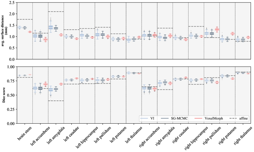
The metrics show significant improvement over affine registration on most subcortical structures. The differences between label uncertainties are less pronounced than between transformation uncertainties. ASDsand DSCsare generally marginally better when using samples from SG-MCMCthan from the approximate variational posterior. Better accuracy in case of SGLDis expected, given restrictive assumptions of the approximate variational model. VI, SG-MCMC, and VoxelMorph produce similar accuracy, despite different uncertainty estimates.
Quantitative comparison of uncertainty estimates. It is difficult to define ground truth uncertainty with regards to image registration. Luo et al. (2019) suggested that well-calibrated image registration uncertainty estimates need to be informative of anatomical features, which are important in neurosurgery. To compare the uncertainty output by different models quantitatively and evaluate whether the uncertainty estimates are clinically useful, we adopt a method similar to that used by Luo et al. (2019) and calculate the Pearson correlation coefficient between the displacement uncertainties and label uncertainties . Here we define label uncertainty to be the standard deviation of the DSCfor each subcortical structure, and displacement uncertainty to be the voxel-wise mean of the displacement field standard deviation magnitude within the region that corresponds to a given subcortical structure.
| model | |
| VI | |
| SG-MCMC | |
| VoxelMorph |
The correlation coefficient is highest in case of VoxelMorph but qualitative evidence suggests that image registration uncertainty output by the model is not well calibrated. The displacement field uncertainty is more informative of label uncertainty in case of SG-MCMCthan VI, so the uncertainty estimates output by SG-MCMCare likely to be more useful for clinical purposes than those output by VIor VoxelMorph.
Transformation smoothness. Finally, in order to evaluate the quality of the model output, in Table 3 we report the number of voxels where the sampled transformations are not diffeomorphic. Each model produces transformations where the number of non-positive Jacobian determinants is nearly zero. SG-MCMCslightly reduced the number of non-positive Jacobian determinants compared to VI. The transformations output by VoxelMorph appear more smooth, which is directly related to the lower transformation uncertainty shown in Figure 3.
| model | % () | |
| VI | ||
| SG-MCMC | ||
| VoxelMorph |
6.3.2 Comparison of the output of SG-MCMC for different initialisations
To study the potential impact of initialisation on the output uncertainty estimates, we analyse the transformations sampled from SGLDrun with different initial velocity fields . We experiment with a sample from VI, a zero velocity field which corresponds to an identity transformation, and a random velocity field sampled from a standard multivariate normal distribution. The first 100,000 samples from each chain are discarded to allow MCMCto reach the stationary distribution, and the two Markov chains are run for one million transitions each, from which we extract 500 total samples at regular intervals.
We observed no strong dependence of the result on the initialisation. The uncertainty values are visually identical to those in Figure 3. The mean voxel-wise discrepancy between the magnitudes of uncertainty estimates is approximately , while the maximum is approximately . This suggests that the Markov chains mix well.
6.3.3 Comparison of the output of SG-MCMC for non-parametric SVFs and SVFs based on B-splines
One of the common features of recent state-of-the-art models for non-rigid registration that enable uncertainty quantification, e.g. Dalca et al. (2018) and Krebs et al. (2019), is an SVFtransformation parametrisation as well as a diagonal covariance matrix of the approximate variational posterior of transformation parameters, which ignores spatial correlations. We showed in Section 6.3.1 that this assumption can lead to diffeomorphic transformations that are not smooth even in case of image registration that is not based on deep learning. Furthermore, previous work on uncertainty quantification in image registration made the assumption of independence between control points but not between directions and used transformation parametrisations that guaranteed smoothness in an implicit manner, e.g. B-splines (Simpson et al., 2012) or Gaussian RBFs(Le Folgoc et al., 2017).
To better understand the impact of transformation parametrisations on uncertainty quantification, we analyse the output transformations and uncertainty estimates when using sparse SVFsbased on cubic B-splines. The control point spacing is set to two or four voxels along each dimension, which gives or . The SGLDstep size is set to , using the heuristic in Section 6.3.
In Figure 6, we show the output uncertainties and sample Jacobian determinants. Using SVFsbased on B-splines results in smoother transformations. In fact, the implicit smoothness of B-splines helps both with the crude assumption of a diagonal covariance matrix in VI, which translates to a diagonal pre-conditioning matrix in SGLD, and with computational and memory efficiency. We also observed a positive impact on the image registration accuracy. For both control point spacings, SVFsbased on B-splines are more accurate than non-parametric SVFson the majority of structures. Despite comparable accuracy, the uncertainty estimates differ.
7 Discussion
7.1 Modelling assumptions
To draw samples from the true posterior of transformation parameters remains a difficult problem even with a large number of simplifying model assumptions. If the true posterior were approximately Gaussian, VIwould provide a good approximation thereof and the lower uncertainty output by SG-MCMCwould indicate that the output samples are autocorrelated even with subsampling. However, if the true posterior is not Gaussian, then the posterior output by VIis ill-fitting, and the samples output by SG-MCMCcover multiple modes near the mode that corresponds to VI, which makes a good case for the use of SGLD.
In practice, the quality of uncertainty estimates is also sensitive to the validity of model assumptions. These include coinciding image intensities up to the expected spatial noise offsets and ignoring spatial correlations between residuals. The first assumption is valid in case of mono-modal registration but the model can be easily adapted to other settings through use of a different data loss. We manage the second assumption by use of virtual decimation (Groves et al., 2011; Simpson et al., 2012), which calculates the effective degrees of freedom of the residual map with stationary covariance by proxy of the correlation between neighbouring voxels in each direction.
We showed how good modelling choices, such as a careful choice of priors and transformation parametrisation can mitigate some of the issues caused by approximations necessary in practical applications. The main problem in inter-subject brain MRIregistration remains accuracy but the trade-off between the quality of the transformation and registration accuracy can be managed effectively.
7.2 Runtime
The experiments were run on a system with an Intel i9-10920X CPU and a GeForce RTX 3090 GPU. Table 4 shows the runtime of the models. VItakes approximately to register a pair of images and produces 140 samples/sec, while SG-MCMCproduces 25 autocorrelated samples/sec. The registration time for SG-MCMCis absent because it is difficult to pin down the mixing time, so a fair comparison of the relative efficiency of VIand SG-MCMCcan be done only on the basis of the number of samples per second.
Due to lack of publicly available information we cannot directly compare the efficiency of our model to other Bayesian image registration methods. The speed of our model is an order of magnitude better than reported by Le Folgoc et al. (2017), while also being three- rather than two-dimensional. Thus, the proposed method based on SG-MCMCis very efficient given the Bayesian constraint. It is not as efficient as feed-forward neural networks, such as VoxelMorph. However, the proposed model is fully Bayesian and enables asymptotically exact sampling from the posterior of transformation parameters.
| model | training time | registration time | samples/sec |
| VI | — | ||
| SG-MCMC | — | — | |
| VoxelMorph |
8 Conclusion
In this paper we presented a new Bayesian model for three-dimensional medical image registration. The proposed regularisation loss allows to adjust regularisation strength to the data when using an SVFtransformation parametrisation, which involves a very large number of degrees of freedom. Sampling from the posterior distribution via SG-MCMCmakes it possible to quantify registration uncertainty even for large images. The computational efficiency and theoretical guarantees regarding samples output by SG-MCMCmake our model an attractive alternative for uncertainty quantification in non-rigid image registration compared to methods based on VI.
Acknowledgments
This research used UK Biobank resources under the application number 12579. Daniel Grzech is funded by the EPSRC CDT for Medical Imaging EP/L015226/1 and Loïc Le Folgoc by EP/P023509/1. We are very grateful to Prof. Wells and the Reviewers for their feedback during the review process.
Ethical Standards
The work follows appropriate ethical standards in conducting research and writing the manuscript, following all applicable laws and regulations regarding treatment of animals or human subjects.
Conflicts of Interest
We declare we do not have conflicts of interest.
References
- Arsigny et al. (2006) Vincent Arsigny, Olivier Commowick, Xavier Pennec, and Nicholas Ayache. A Log-Euclidean Framework for Statistics on Diffeomorphisms. In MICCAI, 2006.
- Ashburner (2007) John Ashburner. A fast diffeomorphic image registration algorithm. NeuroImage, 2007.
- Avants et al. (2014) Brian B. Avants, Nicholas J. Tustison, Michael Stauffer, Gang Song, Baohua Wu, and James C. Gee. The Insight ToolKit image registration framework. Frontiers in Neuroinformatics, 8, 2014.
- Balakrishnan et al. (2018) Guha Balakrishnan, Amy Zhao, Mert R. Sabuncu, John Guttag, and Adrian V. Dalca. An Unsupervised Learning Model for Deformable Medical Image Registration. In CVPR, 2018.
- Balakrishnan et al. (2019) Guha Balakrishnan, Amy Zhao, Mert R. Sabuncu, John Guttag, and Adrian V. Dalca. VoxelMorph: A Learning Framework for Deformable Medical Image Registration. IEEE Transactions on Medical Imaging, 2019.
- Besag (1993) Julian Besag. Comments on ”Representations of knowledge in complex systems” by U. Grenander and MI Miller. Journal of the Royal Statistical Society, 56:591–592, 1993.
- Chen et al. (2016) Changyou Chen, David Carlson, Zhe Gan, Chunyuan Li, and Lawrence Carin. Bridging the Gap between Stochastic Gradient MCMC and Stochastic Optimization. In AISTATS, 2016.
- Dalca et al. (2018) Adrian V. Dalca, Guha Balakrishnan, John Guttag, and Mert R. Sabuncu. Unsupervised Learning for Fast Probabilistic Diffeomorphic Registration. In MICCAI, 2018.
- Dalca et al. (2019) Adrian V. Dalca, Guha Balakrishnan, John Guttag, and Mert R. Sabuncu. Unsupervised Learning of Probabilistic Diffeomorphic Registration for Images and Surfaces. MedIA, 57:226–236, 2019.
- de Vos et al. (2019) Bob D. de Vos, Floris F. Berendsen, Max A. Viergever, Hessam Sokooti, Marius Staring, and Ivana Išgum. A deep learning framework for unsupervised affine and deformable image registration. MedIA, 52:128–143, 2019.
- Delyon et al. (1999) Bernard Delyon, Marc Lavielle, and Eric Moulines. Convergence of a stochastic approximation version of the EM algorithm. Annals of Statistics, 27(1):94–128, 1999.
- Du and Mordatch (2019) Yilun Du and Igor Mordatch. Implicit Generation and Generalization in Energy-Based Models. In NeurIPS, 2019.
- Glocker et al. (2008) Ben Glocker, Nikos Komodakis, Georgios Tziritas, Nassir Navab, and Nikos Paragios. Dense image registration through MRFs and efficient linear programming. MedIA, 12(6):731–741, 2008.
- Groves et al. (2011) Adrian R. Groves, Christian F. Beckmann, Steve M. Smith, and Mark W. Woolrich. Linked independent component analysis for multimodal data fusion. NeuroImage, 54(3):2198–2217, 2011.
- Grzech et al. (2020) Daniel Grzech, Bernhard Kainz, Ben Glocker, and Loïc Le Folgoc. Image registration via stochastic gradient Markov chain Monte Carlo. In UNSURE MICCAI, 2020.
- Hachama et al. (2012) Mohamed Hachama, Agnès Desolneux, and Frédéric J.P. Richard. Bayesian technique for image classifying registration. IEEE Transactions on Image Processing, 21(9):4080–4091, 2012.
- Heinrich (2019) Mattias P. Heinrich. Closing the Gap Between Deep and Conventional Image Registration Using Probabilistic Dense Displacement Networks. In MICCAI, 2019.
- Hill (2020) Mitchell Krupiarz Hill. Learning and Mapping Energy Functions of High-Dimensional Image Data. PhD thesis, UCLA, 2020.
- Janoos et al. (2012) Firdaus Janoos, Petter Risholm, and William Wells. Bayesian characterization of uncertainty in multi-modal image registration. In WBIR, 2012.
- Jordan et al. (1999) Michael I. Jordan, Zoubin Ghahramani, Tommi S. Jaakkola, and Lawrence K. Saul. Introduction to variational methods for graphical models. Machine Learning, 37(2):183–233, 1999.
- Karabulut et al. (2017) Navdar Karabulut, Ertunç Erdil, and Çetin Müjdat. A Markov Chain Monte Carlo based Rigid Image Registration Method. In Signal Processing and Communications Applications Conference, 2017.
- Khawaled and Freiman (2020) Samah Khawaled and Moti Freiman. Unsupervised deep-learning based deformable image registration: A Bayesian framework. In Medical Imaging Meets NeurIPS, 2020.
- Klein et al. (2009) Stefan Klein, Marius Staring, Keelin Murphy, Max A. Viergever, and Josien P.W. Pluim. Elastix: a toolbox for intensity-based medical image registration. IEEE Transactions on Medical Imaging, 29(1):196–205, 2009.
- Krebs et al. (2019) Julian Krebs, Hervé Delingette, Boris Mailhé, Nicholas Ayache, and Tommaso Mansi. Learning a Probabilistic Model for Diffeomorphic Registration. IEEE Transactions on Medical Imaging, 38(9), 2019.
- Le Folgoc et al. (2017) Loïc Le Folgoc, Hervé Delingette, Antonio Criminisi, and Nicholas Ayache. Quantifying Registration Uncertainty With Sparse Bayesian Modelling. IEEE Transactions on Medical Imaging, 36(2):607–617, 2017.
- Lee et al. (2019) Matthew C. H. Lee, Ozan Oktay, Andreas Schuh, Michiel Schaap, and Ben Glocker. Image-and-Spatial Transformer Networks for Structure-Guided Image Registration. In MICCAI, 2019.
- Liu et al. (2019) Lihao Liu, Xiaowei Hu, Lei Zhu, and Pheng Ann Heng. Probabilistic Multilayer Regularization Network for Unsupervised 3D Brain Image Registration. In MICCAI, 2019.
- Luo et al. (2019) Jie Luo, Alireza Sedghi, Karteek Popuri, Dana Cobzas, Miaomiao Zhang, Frank Preiswerk, Matthew Toews, Alexandra Golby, Masashi Sugiyama, William M. Wells III, and Sarah Frisken. On the Applicability of Registration Uncertainty. In MICCAI, 2019.
- Mandt et al. (2017) Stephan Mandt, Matthew D. Hoffman, and David M. Blei. Stochastic Gradient Descent as Approximate Bayesian Inference. Journal of Machine Learning Research, 18:1–35, 2017.
- Modat et al. (2012) Marc Modat, Pankaj Daga, M. Jorge Cardoso, Sebastien Ourselin, Gerard R. Ridgway, and John Ashburner. Parametric non-rigid registration using a stationary velocity field. In Proceedings of the Workshop on Mathematical Methods in Biomedical Image Analysis, 2012.
- Neal (2011) Radford M. Neal. MCMC Using Hamiltonian Dynamics, chapter 5. CRC Press, 2011.
- Neuberger et al. (1997) J. W. Neuberger, A. Dold, and F. Takens. Sobolev Gradients and Differential Equations. Lecture Notes in Computer Science. Springer, 1997.
- Niethammer et al. (2019) Marc Niethammer, Roland Kwitt, and François-Xavier Vialard. Metric Learning for Image Registration. In CVPR, 2019.
- Nijkamp et al. (2019) Erik Nijkamp, Mitch Hill, Song-Chun Zhu, and Ying Nian Wu. Learning Non-Convergent Non-Persistent Short-Run MCMC Toward Energy-Based Model. In NeurIPS, 2019.
- Richard et al. (2009) Frédéric J.P. Richard, Adeline M.M. Samson, and Charles A. Cuénod. A SAEM algorithm for the estimation of template and deformation parameters in medical image sequences. Statistics and Computing, 19(4):465–478, 2009.
- Risholm et al. (2010) Petter Risholm, Steve Pieper, Eigil Samset, and William M. Wells. Summarizing and visualizing uncertainty in non-rigid registration. In MICCAI, 2010.
- Risholm et al. (2011) Petter Risholm, James Balter, and William M. Wells III. Estimation of Delivered Dose in Radiotherapy: The Influence of Registration Uncertainty. In MICCAI, 2011.
- Risholm et al. (2013) Petter Risholm, Firdaus Janoos, Isaiah Norton, Alex J. Golby, and William M. Wells. Bayesian characterization of uncertainty in intra-subject non-rigid registration. MedIA, 2013.
- Rueckert et al. (1999) Daniel Rueckert, L. I. Sonoda, C. Hayes, D. L. G. Hill, M. O. Leach, and David J. Hawkes. Nonrigid registration using free-form deformations: Application to breast MR images. IEEE Transactions on Medical Imaging, 18(8):712–721, 1999.
- Schnabel et al. (2001) Julia A. Schnabel, Daniel Rueckert, Marcel Quist, Jane M. Blackall, Andy D. Castellano-Smith, Thomas Hartkens, Graeme P. Penney, Walter A. Hall, Haiying Liu, Charles L. Truwit, Frans A. Gerritsen, Derek L. G. Hill, and David J. Hawkes. A Generic Framework for Non-rigid Registration Based on Non-uniform Multi-level Free-Form Deformations. In MICCAI, 2001.
- Schultz et al. (2018) Sandra Schultz, Heinz Handels, and Jan Ehrhardt. A multilevel Markov Chain Monte Carlo approach for uncertainty quantification in deformable registration. In SPIE Medical Imaging, 2018.
- Schultz et al. (2019) Sandra Schultz, Julia Krüger, Heinz Handels, and Jan Ehrhardt. Bayesian inference for uncertainty quantification in point-based deformable image registration. In SPIE Medical Imaging, 2019.
- Sedghi et al. (2019) Alireza Sedghi, Tina Kapur, Jie Luo, Parvin Mousavi, and William M. Wells. Probabilistic Image Registration via Deep Multi-class Classification: Characterizing Uncertainty. In UNSURE MICCAI, 2019.
- Shen et al. (2019) Zhengyang Shen, François Xavier Vialard, and Marc Niethammer. Region-specific diffeomorphic metric mapping. In NeurIPS, 2019.
- Sherman and Morrison (1950) Jack Sherman and Winifred J. Morrison. Adjustment of an Inverse Matrix Corresponding to Changes in the Elements of a Given Column or a Given Row of the Original Matrix. The Annals of Mathematical Statistics, 21(1):124–127, 1950.
- Simpson et al. (2015) I. J.A. Simpson, M. J. Cardoso, M. Modat, D. M. Cash, M. W. Woolrich, J. L.R. Andersson, J. A. Schnabel, and S. Ourselin. Probabilistic non-linear registration with spatially adaptive regularisation. MedIA, 26(1):203–216, 2015.
- Simpson et al. (2012) Ivor J.A. Simpson, Julia A. Schnabel, Adrian R. Groves, Jesper L.R. Andersson, and Mark W. Woolrich. Probabilistic inference of regularisation in non-rigid registration. NeuroImage, 59(3):2438–2451, 2012.
- Simpson et al. (2013) Ivor J.A. Simpson, Mark W. Woolrich, Jesperl R. Andersson, Adrian R. Groves, and Julia Schnabel. Ensemble learning incorporating uncertain registration. IEEE Transactions on Medical Imaging, 32(4):748–756, 2013.
- Slavcheva et al. (2018) Miroslava Slavcheva, Maximilian Baust, and Slobodan Ilic. SobolevFusion: 3D Reconstruction of Scenes Undergoing Free Non-rigid Motion. In CVPR, 2018.
- Sudlow et al. (2015) Cathie Sudlow, John Gallacher, Naomi Allen, Valerie Beral, Paul Burton, John Danesh, Paul Downey, Paul Elliott, Jane Green, Martin Landray, et al. Uk biobank: An open access resource for identifying the causes of a wide range of complex diseases of middle and old age. PLOS Medicine, 12(3), 2015.
- Wassermann et al. (2014) Demian Wassermann, Matt Toews, Marc Niethammer, and William Wells III. Probabilistic Diffeomorphic Registration: Representing Uncertainty. In WBIR, 2014.
- Welling and Teh (2011) Max Welling and Yee Whye Teh. Bayesian Learning via Stochastic Gradient Langevin Dynamics. In ICML, 2011.
- whuber (2018) whuber. What is the expected value of the logarithm of gamma distribution?, Oct 2018. URL https://stats.stackexchange.com/questions/370880/what-is-the-expected-value-of-the-logarithm-of-gamma-distribution.
- Zhang and Fletcher (2014) Miaomiao Zhang and P. Thomas Fletcher. Bayesian principal geodesic analysis in diffeomorphic image registration. In MICCAI, 2014.
- Zhang et al. (2013) Miaomiao Zhang, Nikhil Singh, and P. Thomas Fletcher. Bayesian Estimation of Regularization and Atlas Building in Diffeomorphic Image Registration. In IPMI, 2013.
- Zhang et al. (2020) Ruqi Zhang, Chunyuan Li, Jianyi Zhang, Changyou Chen, and Andrew Gordon Wilson. Cyclical stochastic gradient MCMC for bayesian deep learning. In ICLR, 2020.
- Zöllei et al. (2007) Lilla Zöllei, Mark Jenkinson, Samson Timoner, and William Wells. A marginalized MAP approach and EM optimization for pair-wise registration. In IPMI, 2007.
A
In this appendix we show how to calculate the mean of the logarithm of the gamma distribution (whuber, 2018).
Let be a random variable which follows the gamma distribution with the shape and rate parameters and , i.e. . We are interested in the expected value of . If we assume that , then the PDFof is given by:
| (16) |
Note that is a constant and the integral of must equal , so we have:
| (17) |
Let . This means that , so the PDFof is given by:
| (18) |
Again, because is a constant and the integral of the PDFof must equal , we have:
| (19) |
Now, using Feynman’s trick of differentiating under the integral sign, we see that:
| (20) | |||||||||
| (21) | |||||||||
| (22) | |||||||||
| (23) | |||||||||
where is the digamma function. Finally, the rate parameter shifts the logarithm by . Therefore, the expected value of is given by:
| (24) |
B
In this appendix we show how to calculate the KL-divergenceterm between the approximate variational posterior and the prior , as well as the entropy of the approximate variational posterior, both of which are needed to maximise the ELBOin Equation 12.
The KL-divergencecan be evaluated in terms of the entropy of the approximate variatonal posterior and the regularisation energy :
| (25) |
where denotes the expected value.
The entropy of the approximate variational posterior is calculated as follows:
| (26) |
The first term on the left on the RHS is calculated using the matrix determinant lemma:
| (27) |
To evaluate the other term, and in particular the precision matrix , we can use the Sherman-Morrison formula (Sherman and Morrison, 1950), which states that:
| (28) |