Tractography is one way to represent a structural connectome, or structural network of a brain, which consists of brain regions that are physically connected by a network of neuronal bundles that make up the white matter of that brain. It is not currently possible to image individual neurons in a living brain non-invasively. Instead, we can use diffusion-weighted magnetic resonance images (DWMRI) to infer the pathways of coherent bundles of neurons that cross through other bundles in white matter and connect with end points in gray matter. There are a variety of tractography algorithms used to infer these white matter pathways, ranging from local methods that integrate local orientation information to form individual streamlines to global methods that estimate all fiber tracts simultaneously. Deterministic (basser2000vivo) and probabilistic (behrens2003characterization) streamline integration methods are easy to compute, but they suffer from accumulation of local orientation errors leading to tract reconstructions biased toward shorter and straighter tracts. Conversely, global estimation methods (jbabdi2007bayesian; christiaens2015global) incorporate prior anatomical knowledge while ensuring that tractography is consistent with the underlying data. However, these global methods have convergence issues, sensitivity to initialization and priors, and a tendency to have estimated tracts end in the middle of white matter regions. Biases in tract reconstruction introduced by either local or global methods affect the accuracy of quantitative measures such as track density and connection strength.

Geodesic tractography algorithms, first introduced by o2002new, use a combination of local and global information to determine tracts by formulating white matter pathways as geodesic curves under a Riemannian metric derived from the DWMRI data. In the original work, o2002new use the inverse diffusion tensor as the Riemannian metric. As described by lenglet2004, the inverse diffusion tensor metric has a connection to Brownian motion through the Laplace Beltrami operator on the resulting Riemannian manifold. The inverse tensor metric favors paths that follow the principal eigenvector of the diffusion tensor, as this is the locally optimal direction to move. However, geodesic curves for this metric do not consistently follow the principal eigenvector of the diffusion tensor, and tend to be overly straight in regions where the white matter fibers are bending, losing association with the underlying anatomy in these areas. This problem has been addressed by several strategies to improve the adherence of geodesics to the white matter geometry, including “sharpening” the inverse diffusion tensor (fletcher2007), using the adjugate of the diffusion tensor (fuster2016), and using a conformal metric (hao2014improved). One advantage to the geodesic tractography formulation is that we can do uncertainty and confidence interval analysis of the tractographies following (sengers2021).

These tractography techniques help to give insight into the structure of a single brain, but it remains an open challenge to quantitatively measure how these structural connectome pathways vary in a population. To do such a population analysis, we first need a common frame of reference, or atlas space, where spatial differences between subjects’ white matter can be measured.

Initially, white matter atlases were constructed by aligning DWMRI to an anatomical template, then transforming and averaging the associated tensor field or distribution function field. For example, mori2008dti construct a diffusion tensor imaging (DTI) atlas by registering the DWMRI of multiple subjects to a standardized anatomical template. They build the DTI atlas by transforming the diffusion tensors for each subject (alexander2001spatial) and then taking the Euclidean average of the transformed diffusion tensors at each voxel. This approach does not use the white matter directionality information encoded in the diffusion images during the registration. It also suffers from the fact that the Euclidean average of diffusion tensors does not take into account the directionality and tends to be fatter (i.e., less anisotropic) than the input tensors (fletcher2007riemannian). Another approach by yeh2018population is to register $q$-space diffusion images into an anatomical template and estimate the spin distribution function (SDF) at each voxel in the template. Then the SDFs are averaged on a per-voxel basis. While this method does take into account the directionality of the white matter in a local neighborhood, it does not take into account consistency of long-range white matter connections. These methods both rely on low-accuracy registration to the anatomical template image, because at the time high-accuracy diffeomorphic registrations could not be used as they did not preserve the continuity of pathway directions across voxels (yeh2018population).

The field then focused on constructing atlases directly from tractography. These methods are adept at finding well-known tracts, but they generally require significant expert curation to remove the many false-positive fibers and tracts they create (zhang2018anatomically). Additionally, variation of population-level tractography characteristics like fiber density of tracts is as likely to be reflective of the tractography process chosen as it is of the underlying physical white matter. These and other biases in tractography quantification are well-characterized by jeurissen2019diffusion.

In order to get a more complete anatomical atlas,  toga2006towards argue for the integrated derivation of multimodal atlases using techniques such as spatial normalization to produce more comprehensive atlases. Some attempts have been made to create a multimodal population atlas from T1 and DWMRI images. gupta2016framework rigidly register the DWMRI into the same space as the T1 template image and then apply the same deformations used to create the T1 template to the DWMRI before estimating the diffusion tensors from the transformed DWMRI. This approach puts the DWMRI and T1 images in the same space, but does not use the white matter structure to inform the creation of the T1 atlas. Other previous work on multichannel registration of diffusion and T1 MRI include avants2007multivariate, who use a Euclidean image match metric on the diffusion tensors, and uus2020multi, who use local angular correlation on the orientation distribution functions (ODFs). Like the white matter-only atlases approaches discussed above, these methods only take local information into consideration and thus do not preserve the consistency of long-range white matter connections. They do demonstrate that registration quality is improved over single channel registration when complementary channels are combined in the objective function.

We are motivated to find an approach that can preserve the best aspects of these atlas and tractography methods, while mitigating their weaknesses. Specifically, we want to create a white matter pathway atlas that preserves local orientations and other anatomical information while maintaining the continuity and integrity of long-range connections. We then want a method to bring subjects into that atlas space to enable statistical quantification of both structural connectivity and geometric variability of white matter structure across a population.

To meet these goals, we describe the metric matching framework presented by campbell2021structural in more detail and then extend it by combining diffeomorphic metric matching with diffeomorphic image matching to enable the construction of both a multimodal white and gray matter atlas simultaneously for the first time. This formulation preserves geodesics transformed by diffeomorphisms, which meets our objective to use local diffusion data and maintain the integrity of long-range connectomics as inferred by tractography (cheng2015tractography). We demonstrate that long-range connections are preserved by performing geodesic tractography on the resulting atlas.

In the white matter of the brain, the diffusion of water is restricted perpendicular to the direction of the axons. Diffusion-weighted MRI measures the microscopic diffusion of water in multiple directions at every voxel in a 3D volume. Thus, the directionality of white matter in the brain can be locally inferred. Traditionally, global connections of the white matter have been estimated by a procedure called tractography, which numerically computes integral curves of the vector field formed by the most likely direction of fiber tracts at each point. DTI models anisotropic water diffusion with a 3x3 symmetric positive definite tensor, $D(x)$, at each voxel, $x\in M$, where the manifold $M\subset\mathbb{R}^{3}$ is the image domain. The principal eigenvector of $D(x)$ is aligned with the direction of the strongest diffusion.

Riemannian metrics that represent connectomics of a subject have been developed in diffusion imaging by  o2002new and include the inverse-tensor metric $\tilde{g}=D(x)^{-1}$. However, the geodesics associated with the inverse-tensor metric tend to deviate from the principal eigenvector directions and take straighter paths through areas of high curvature.

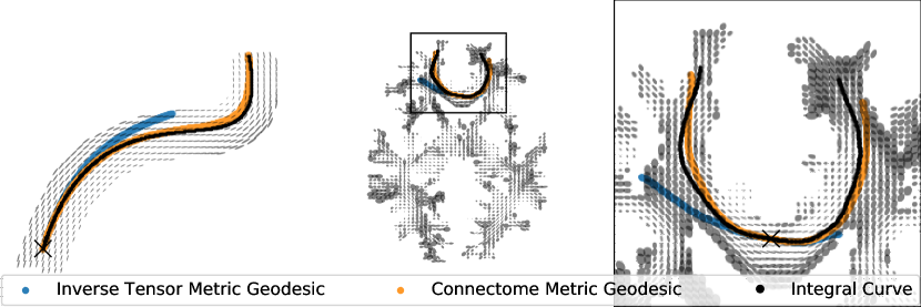
In this work we build on the algorithm developed by hao2014improved, which estimates a spatially-varying function, $\alpha(x):M\to\mathbb{R}$, that modulates the inverse-tensor metric to create a locally-adaptive Riemannian metric, $g_{\alpha}=e^{\alpha(x)}\tilde{g}$. We briefly describe the method here for completeness but refer the reader to hao2014improved for details. This adaptive connectome metric, $g_{\alpha}$, is conformally equivalent to the inverse-tensor metric and is better at capturing the global connectomics, particularly through regions of high curvature. Figure 1 shows how well the geodesics of each metric match the integral curve of the vector field. The connectome metric geodesics are very closely aligned with the integral curves.

The geodesic between two end-points, $p,q\in M$, associated with the inverse-tensor metric, $\tilde{g}(x)=D(x)^{-1}$, minimizes the energy functional, $\tilde{E}$, while the geodesic associated with the connectome metric, $g_{\alpha}(x)=e^{\alpha(x)}D(x)^{-1}$, minimizes the energy functional, $E_{\alpha}$.

where $\gamma:[0,1]\to M$, $\gamma(0)=p$, $\gamma(1)=q$, $T=\frac{d\gamma}{dt}$.

Analyzing the variation of $E_{\alpha}$ leads to the geodesic equation, $\mathrm{grad}\,\alpha=2\nabla_{T}T$, where the Riemannian gradient of $\alpha$, $\mathrm{grad}\,\alpha=\tilde{g}^{-1}\bigl{(}\frac{\partial\alpha}{\partial x^{$, and $\nabla_{T}T$ is the covariant derivative of $T$ along its integral curve.

To enforce the desired condition where the tangent vectors, $T$, of the geodesic match the vector field, $V$, of the unit principal eigenvectors of $D(x)$, we minimize the functional, $F(\alpha)=\int_{M}||\mathrm{grad}\,\alpha-2\nabla_{V}V||^{2}_{\tilde{g}}dx$. The equation for $\alpha$ that minimizes $F(\alpha)$ is

where $\mathrm{div}$ and $\Delta$ are the Riemannian divergence and Laplace-Beltrami operator. We discretize the Poisson equation in Equation (2) using a second-order finite difference scheme that satisfies both the Neumann boundary conditions $\frac{\partial\alpha}{\partial\overrightarrow{n}}=\langle\mathrm{grad}\,\alpha$ and the governing equation on the boundary. We then solve for $\alpha$.

Note that we can use this method to match the geodesics of the connectome metric to other vector fields defining the tractogram, e.g., from higher-order diffusion models that can represent multiple fiber crossings in a voxel. In particular, for tractography based on fiber orientation distributions (FODs), we can use the techniques presented in nie2019topographic to generate the vector field $V$.

The fundamental result of the purposed method is the fact that a metric tensor field is estimated such that a given vector field is a geodesic vector field of the estimated Riemannian metric. It is in this sense that the estimated metric field captures the geometry of the white matter as inferred by tractoraphy. This metric field that captures the tractography will be the primary driving force for the registration algorithms. We will now develop registration and atlas construction algorithms that leverage the rich geometric structure of Manifold of all Riemannian Metrics.

Once we have estimated a Riemannian metric for a human connectome, it is a point in the infinite-dimensional manifold of all Riemannian metrics, $\operatorname{Met}(M)$, where $M$ is the domain of the image. We will equip this space with a diffeomorphism-invariant Riemannian metric, called the Ebin or DeWitt metric (Ebin1970a; DeWitt67). The invariance of the infinite-dimensional metric under the group of diffeomorphisms $\operatorname{Diff}(M)$ is a crucial property, as it guarantees the independence of an initial choice of coordinate system on the brain manifold. As we will base our statistical framework on this infinite-dimensional geometric structure, we will now give a detailed overview of its induced geometry on $\operatorname{Met}(M)$.

Let $M$ be a smooth $n$-dimensional manifold; for our targeted applications $n$ will be two or three. We denote by $\operatorname{Met}(M)$ the space of all smooth Riemannian metrics on $M$, i.e., each element $g$ of the space $\operatorname{Met}(M)$ is a symmetric, positive-definite $0\choose 2$ tensor field on $M$. It is convenient to think of the elements of $M$ as being point-wise positive-definite sections of the bundle of symmetric two-tensors $S^{2}T^{\ast}M$, i.e., smooth maps from $M$ with values in $S^{2}_{+}T^{\ast}M$. Thus, the space $\operatorname{Met}(M)$ is an open subset of the linear space $\Gamma(S^{2}T^{\ast}M)$ of all smooth symmetric $0\choose 2$ tensor fields and hence itself a smooth Fréchet-manifold (Ebin1970a). Furthermore, let $\operatorname{Diff}(M)$ denote the infinite-dimensional Lie group of all smooth diffeomorphisms of the manifold $M$. Elements of $\operatorname{Diff}(M)$ act as coordinate changes on the manifold $M$. This group acts on the space of metrics via pullback

In an analogous way we can define the pushforward action

It is important to note that the geometries of the metrics $g$ and $\varphi^{*}g$ ($\varphi_{*}g$ resp.) are also related via $\varphi$. In particular, geodesics with respect to $g$ are mapped via $\varphi$ to geodesics with respect to $\varphi^{*}g$ (via $\varphi^{-1}$ for $\varphi_{*}g$, resp.). On the infinite-dimensional manifold $\operatorname{Met}(M)$, there exists a natural Riemannian metric: the reparameterization-invariant $L^{2}$-metric. To define the metric, we need to first characterize the tangent space of the manifold of all metrics: $\operatorname{Met}(M)$ is an open subset of $\Gamma(S^{2}T^{\ast}M)$. Thus, every tangent vector $h$ is a smooth bilinear form $h:TM\times_{M}TM\to{\mathbb{R}}$ that can be equivalently interpreted as a map $TM\to T^{\ast}M$. The $L^{2}$-metric is given by

with $g\in\operatorname{Met}(M)$, $h,k\in T_{g}\operatorname{Met}(M)$ and $\operatorname{vol}(g)$ the induced volume density of the metric $g$. This metric, introduced in Ebin1970a, is also known as the Ebin metric. We call the metric natural as it requires no additional background structure and is consequently invariant under the pushforward and pullback actions of the diffeomorphism group, i.e.,

for all $\varphi\in\operatorname{Diff}(M)$, $g\in\operatorname{Met}(M)$ and $h,k\in T_{g}\operatorname{Met}(M)$. Note that the invariance of the metric follows directly from the substitution formula for multi-dimensional integrals.

The Ebin metric induces a particularly simple geometry on the space $\operatorname{Met}(M)$, with explicit formulas for geodesics, geodesic distance and curvature. In the following theorem and corollary, we will present the most important of these formulas, which will be of importance for our proposed metric matching framework.

First we note that a metric $g\in\operatorname{Met}(M)$, in local coordinates, can be represented as a field of symmetric, positive-definite $n\times n$ matrices that vary smoothly over $M$. Similarly, each tangent vector at $g$ can be represented as a field of symmetric $n\times n$ matrices. By the results of freed1989basic; gil1991riemannian; clarke2013geodesics, one can reduce the investigations of the space of all Riemannian metrics to the study of the geometry of the finite-dimensional space of symmetric, positive-definite $n\times n$ matrices. The point-wise nature of the Ebin metric allows one to solve the geodesic initial and boundary value problem on $\operatorname{Met}(M)$ for each $x\in M$ separately. Consequently the formulas for geodesics, geodesic distance and curvature on the finite-dimensional matrix space can be translated directly to results for the Ebin metric on the infinite-dimensional space of Riemannian metrics.

Note that the space of Riemannian metrics, $\operatorname{Met}(M)$ with the Ebin metric, is not metrically complete and not geodesically convex. Thus the minimal geodesic between two Riemannian metrics may not exist in $\operatorname{Met}(M)$, but only in a larger space; the metric completion $\overline{\operatorname{Met}}(M)$, which consists of all possibly degenerate Riemannian metrics. This construction has been worked out in detail by clarke2013completion – including the existence of minimizing paths in $\overline{\operatorname{Met}}(M)$. In the following proof, we will omit these details and refer the interested reader to the article clarke2013completion for a more in-depth discussion. In Theorem 1, we present an explicit formula for the minimizing geodesic in $\overline{\operatorname{Met}}(M)$ that connects two given Riemannian metrics.

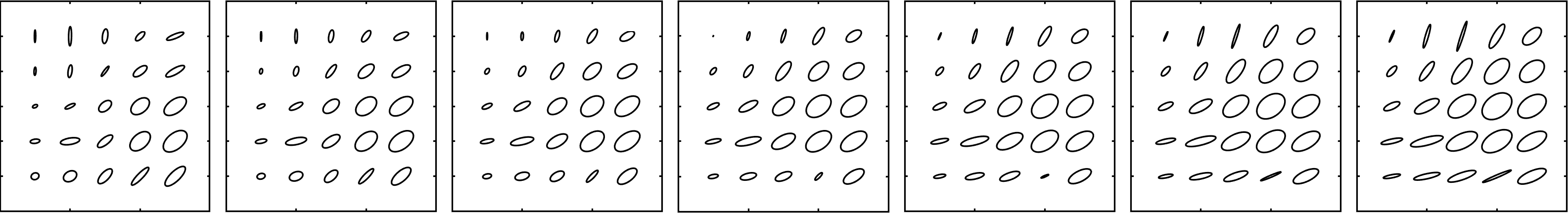
An example of calculating a geodesic in the space $\overline{\operatorname{Met}}(M)$ using the explicit formula is visualized in Figure 2. The ellipse in the fifth row and fourth column, and the one in the first column and row of this figure are examples of geodesic paths that include possibly degenerate Riemannian metrics from the completion $\overline{\operatorname{Met}}(M)$. Note that handling these degenerate cases are well understood and we did not observe any numerical issues associated with such cases.

Next, we recall that the geodesic distance of a Riemannian metric is defined as the infimum of all paths connecting two given points,

where the infimum is taken over all paths $g:[0,1]\to\operatorname{Met}(M)$ with $g(0)=g_{0}$ and $g(1)=g_{1}$. As a direct consequence of Theorem 1, we obtain the explicit formula for the distance function given in Corollary 2.

Having equipped the space of Riemannian metrics with the distance function (13), we can consider the Fréchet mean, $\hat{g}$, of a collection of metrics, $g_{1},\ldots g_{N}$, which is defined as a minimizer of the sum of squared distances.

One could directly minimize this functional using a gradient-based optimization procedure. As our distance function is the geodesic distance function of a Riemannian metric and since we have access to an explicit formula for the minimizing geodesics, we will instead use the iterative geodesic marching algorithm, see e.g. ho2013recursive, to approximate the Fréchet mean: Given $N$ Riemannian metrics $g_{i}$, we approximate the Fréchet mean via $\hat{g}=\hat{g}_{N}$, where $\hat{g}_{i}$ is recursively defined as $\hat{g}_{0}=g_{0}$, $\hat{g}_{i}(x)=g(1/(i+1),x)$ and where $g(t,x)$ is the minimal path, as given in Theorem 1, connecting $\hat{g}_{i-1}$ to the $i$-th data point $g_{i}$. Thus one only has to calculate $N$ geodesics in total in the space of Riemannian metrics, whereas a gradient-based algorithm would require one to calculate $N$ geodesic distances in each step of the gradient descent.

Fundamental to the precise characterization and comparison of the human connectome of an individual subject or a population as a whole is the ability to map or register two different human connectomes. The framework of Large Deformation Diffeomorphic Metric Mapping (LDDMM) is well developed for registering points (joshi2000landmark), curves (glaunes2008large) and surfaces (vaillant2005surface) all modeled as submanifolds of ${\mathbb{R}}^{3}$ as well as images modeled as an $L^{2}$ function (beg2005computing).This framework has also been extended to densities (bauer2015diffeomorphic) modeled as volume forms. We now extend the diffeomorphic mapping framework to the connectome modeled as Riemannian metrics. The diffeomorphism group deforms the domain, $M$, and acts naturally on the space of metrics, $\operatorname{Met}(M)$, see Equation (4). With this action and a reparameterization-invariant metric, the problem of registering two connectomes fits naturally into the framework of computational anatomy.

Now the registration of two connectomes is achieved by minimizing the energy

over all such diffeomorphisms in $\operatorname{Diff}(M)$. Here $\operatorname{dist}_{\operatorname{Diff}}$ is a right invariant distance on $\operatorname{Diff}$ and $\operatorname{dist}_{\operatorname{Met}}$ is a reparameterization-invariant distance on the space of all Riemannian metrics, e.g., the geodesic distance of the metrics studied above. The first term measures the deformation cost and the second term is a similarity measure between the target and the deformed source connectome. The invariance of the two distances is essential for the minimization problem to be independent of the choice of coordinate system on the brain manifold.

We use the distance function as introduced in Section 3.1 to measure the deformation cost, i.e., $\operatorname{dist}_{\operatorname{Diff}}(\operatorname{id},\varphi)=$ where $g$ is the restriction of the Euclidean metric to the brain domain. This choice greatly increases computational efficiency since we can now use the formulas from Section 3 as explicit formulas for both terms of the energy functional. To minimize the energy functional, we use a gradient flow approach described in Algorithm LABEL:algo1, where the gradient on $\operatorname{Diff}(M)$ is calculated with respect to a right invariant Sobolev metric of order one, which at the identity is given by

where $\lambda>0$ is a weight parameter, $g$ is the restriction of the Euclidean metric to the brain domain and $\xi_{1},\ldots\xi_{k}$ is an orthonormal basis of the harmonic vector fields on $M$. This metric, sometimes called the information metric, has been first introduced by Modin2015; see also bauer2015diffeomorphic. We choose this specific gradient because of the relation of the information metric to both the Ebin metric on the space of metrics and the Fisher-Rao metric on the space of probability densities. We summarize the relations between these geometries in Figure LABEL:fig:DiffMetCommute; for a precise description of the underlying geometric picture we refer to KLMP2013 and bauer2015diffeomorphic.