1 Introduction
The term Fetal Growth Restriction (FGR) is used to describe a fetus that has not reached their genetic growth potential, due to placental insufficiency causing inadequate supply of oxygen and nutrients (Lyall et al. (2013)). FGR is a clinical diagnosis, defined by the Delphi consensus standardised definitions (Gordijn et al. (2016a)), and is divided into two different phenotypes, with onset either early (less than 32 weeks gestational age (GA)) or late in gestation. It is associated with high rates of stillbirth (Gardosi et al. (2013)), and neonatal morbidity including increased rates of cerebral palsy, bronchopulmonary dysplasia, and cardiovascular disease long term (Colella et al. (2018)). There is currently no treatment for FGR, therefore clinicians must weigh the risks of prematurity against the risk of hypoxia and death in utero to determine the optimal delivery time. There are limited clinical tools to do this, so at present, clinicians follow national guidelines to make this decision (No (2002)).
Considering the complicated nature of treatment and management, understanding the role and development of each organ during FGR is key for effective diagnosis and patient-specific severity assessment of the condition. Studies up to date only include quantitative analysis of a single fetal organ, most commonly the placenta, fetal brain, and fetal liver (Salavati et al. (2019); Malhotra et al. (2017); Miller et al. (2016); Chang et al. (2006); Ebbing et al. (2009)). Our research overcomes these limitations by incorporating a multi-organ analysis for FGR assessment from MRI scans.
MRI is increasingly used to image the placental circulation. The Diffusion-rElaxation Combined Imaging for Detailed Evaluation (DECIDE) multi-compartment model separates fetal and maternal flow characteristics of the placenta allowing measurement of the relative proportions of vascular spaces (Melbourne et al. (2019); Couper et al. (2020)). When applied in early-onset FGR, it identified reduced feto-placental blood oxygen saturation, where the degree of abnormality correlated with disease severity defined by ultrasound fetal and maternal arterial Doppler findings (Aughwane et al. (2020b)).
The motivation for this research was to compare MR derived parameters relating to perfusion and oxygenation within the placenta and three fetal organs (the brain, liver and lungs) between normally grown pregnancies and those complicated by early-onset FGR, through multi-compartment models and texture analysis. This research serves as a preliminary investigation into statistical methods leveraging multi-contrast MRI techniques to identify FGR predictors and thereby predict FGR, its severity, and resulting clinical complications. We propose a set of standardised imaging tools, important features, and initial statistical approaches for use in larger studies. Distinguishing features were then used to predict FGR diagnosis and GA at delivery via simple machine learning models.
2 Related Works
2.1 Single- & Multi-Compartment Models
Blood oxygenation level-dependent (BOLD) contrast is a -weighted sequence. It is affected by variations in concentration of vascular oxygentation in the blood volume and magentic field inhomogeneities. Quantifying enables the determination of oxygen saturation by leveraging the relationationship between and deoxyhemoglobin (Sinding et al. (2016, 2017)). In FGR pregnancies, the placenta is hypoxic, displaying a reduced value which can be used as an FGR biomarker (Robinson et al. (1998); Jiang et al. (2013)). Despite the potential of BOLD-MRI in measuring oxygen saturation, its use has not yet been validated in diagnosis of FGR and interpretation of the placental BOLD signal is complicated by several factors that influence changes in the signal (Sinding et al. (2018); Uğurbil et al. (2000); Chalouhi and Salomon (2014); Sørensen et al. (2015); Turk et al. (2020)). Considering this, and due to the requirements of a gradient echo acquisition, relaxometry is not quantified in the current research.
Instead, T relaxometry provides structural, functional, and morphological tissue information as T transverse relaxation times depend on several factors encompassing water binding, macromolecular concentration, and most importantly, blood oxygenation levels (Derwig et al. (2013); Saini et al. (2020)). Previous literature has shown that the placental T times in SGA or FGR pregnancies are reduced with respect to normal pregnancies (Derwig et al. (2013)). T relaxation times have been used to assess placental function in various applications (Melbourne et al. (2019, 2016a); Jacquier and Salomon (2021); Stout et al. (2021)).
This study extended on previous placental research by producing T maps for different fetal organs. It was hypothesised that because of the brain-sparing effect, certain organs would have lower oxygen levels in FGR compared to healthy pregnancies, and thus reduced T measurements would be extracted from blood flowing through non-prioritised organs in FGR pregnancies. Portnoy et al. demonstrated the precise relationship between blood T relaxation times and oxygen saturation (Portnoy et al. (2017)) by making use of the Luz-Meiboom model, given by Equation 1, presenting the exponential relationship,
| (1) |
where , is the erythrocyte (red blood cell) relaxation rate that depends on oxygen saturation, is the hematocrit (proportion of red blood cells in blood), and is the plasma relaxation rate.
Diffusion-weighted (DW) MRI is a valuable method for investigating the fetal brain-sparing effect; providing measures of brain maturation and detection of brain lesions (Arthurs et al. (2017)). This is attained by measuring water diffusion, which yields corresponding apparent diffusion coefficient (ADC) values. Arthurs et al. established differences between healthy and severe FGR fetuses, frequently leading to the clinical decision of early delivery induction in the latter group (Arthurs et al. (2017)). The time between the MRI examination and delivery was, on average, 7.69 weeks earlier for the FGR group compared to the healthy, thus highlighting the potential of DW-MRI for accurate diagnosis of growth restricted cases - allowing for appropriate management plans to be put in place.
Dynamic contrast-enhanced (DCE) MRI can spatially and quantitatively characterise maternal perfusion of placental insufficiency and tissue vasculature (Ingram et al. (2018); Schrauben et al. (2019); Frias et al. (2015)). It describes the delivery of contrast agent to the maternal side and its transfer into the fetal blood pool in order to distinguish between individual vascular units of the placenta. DCE-MRI is the current gold standard for quantitative descriptions of vascular function (Frias et al. (2015); Schabel et al. (2016)). Nonetheless, this technique has significant drawbacks as it requires an exogenous contrast. The clearance of contrast from the feto-placental system still requires further research. To that end, an imaging technique which does not include any safety concerns for the mother and fetus is more pertinent.
Multi-compartment models refer to advanced mathematical models that separate the signal contributions from different tissue types (Aughwane et al. (2020b)). Diffusion-relaxation models are growing in popularity and have found multiple applications such as in neuroimaging (Kim et al. (2017)), and more recently in placental imaging, encompassing the assessment of placental function in FGR (Melbourne et al. (2019, 2016a); Hutter et al. (2019); Jacquier and Salomon (2021)). A thorough overview of these techniques is provided in (Slator et al. (2021)).
The DECIDE model identifies and separates the values corresponding to the fetal and maternal blood, enabling the quantification of fetal blood oxygen saturation. The precise mechanisms and assumptions describing the DECIDE and the Extended Intravoxel Incoherent Motion Model (IVIM) models are discussed in Section 3.2.
2.2 Diagnosis Predictions using Machine Learning
Supervised Machine Learning (ML) refers to the employment of a predictive model with an assumed relationship between the input (features) and output (labels) variables. Its prominence in medical imaging has been significantly established in recent years, particularly in computer-aided diagnosis (Erickson et al. (2017); Giger (2018)), due to the rise of ‘Big Data’ and available computer power. Its contribution to “intelligent imaging” is by virtue of its potential to advance and enhance detection and diagnosis of complex disorders, risk assessment, and therapy response (Schoepf et al. (2007); Dundar et al. (2008); Summers (2010); Mitchell et al. (2008)). The advantages of ML stem from its ability to draw connections and identify patterns between variables, surpassing human perception. However, its attribute as a ‘black-box function’ makes it difficult to interpret the results from ML models and determine how features are used to arrive at predictions, thus ensuing in a lack of clinician trustworthiness in the models. Nonetheless, ML can be leveraged to assimilate information from datasets where the relationship between the input and output variables are unknown and to select the best features for a certain prediction. It can be used for decision support by aiding clinicians in interpreting medical imaging findings rather than relying entirely on the model predictions alone.
ML enables the consolidation and unravelling of complex biomedical and healthcare data that overcomes the limitations of traditional statistical methods. The aim of these algorithms is to provide solutions to clinical problems by learning statistical associations of the features extracted from the images (Shen et al. (2017)).
Current screening and diagnostic tools for FGR remain suboptimal (Audette and Kingdom (2018)). Delivery of improved clinical outcomes requires greater understanding of the multifactorial pathogenesis in early-onset FGR and distinguishing features or biomarkers of the condition (Audette and Kingdom (2018)). Analysis of a combination of multiple FGR indicators (Gordijn et al. (2018, 2016b); Beune et al. (2018)), can be achieved through use of ML methods. Supervised ML models are increasingly being employed for early prediction and diagnosis of pregnancy conditions, including intrauterine growth restriction, pre-eclampsia, risk of stillbirth, preterm pregnancy, and gestational diabetes (Crockart et al. (2021); Burgos-Artizzu et al. (2020); Caly et al. (2021); Khatibi et al. (2021); Marić et al. (2020); Ye et al. (2020); Koivu and Sairanen (2020)).
Recent work conducted by (Arabi Belaghi et al. (2021)) compared the performance of logistic regression and artificial neural networks in predicting overall and spontaneous preterm birth, on a dataset of 112,963 nulliparous women (singleton gestation) who delivered between 20-42 weeks gestation. The predictors included socio-demographic variables correlated with the risk of preterm birth, such as maternal age, income, education, race, folic acid use, etc. The prediction accuracy of both models in the first trimester was ambiguous. But by incorporating complications during pregnancy as additional predictors, the authors established a 20% increase in the area under the curve (AUC) from the receiver operating characteristic curve (ROC) for artificial neural networks in the validation sample compared to the logistic regressor during the second trimester (80% vs. 60%). The prediction performance of this work cannot be directly compared to our study, given the substantial difference in sample size (being several orders of magnitude smaller), which greatly influences the statistical power of the study. Therefore, our study should be viewed only as a preliminary study, as gaining concrete and detailed information regarding model performance and generalisability, and the features driving each ML model cannot be easily extracted as in (Arabi Belaghi et al. (2021)), where the statistical methods were applied to a much larger dataset.
Research into the prediction of stillbirth by (Yerlikaya et al. (2016)) employed a multivariate logistic regression analysis to deduce the contributions of varying maternal characteristics and medical history in stillbirth prediction. Correspondingly, Trudell et al. generated models for the prediction of stilbirth using backward stepwise logistic regression (Trudell et al. (2017)). Both groups leveraged highly similar maternal demographics and medical history and concluded similar prediction performances ranging between 64% to 67% AUC.
Despite the comparable performance of conventional logistic regression and ML methods for diagnosis predictions in previous literature (Yerlikaya et al. (2016); Trudell et al. (2017); Koivu and Sairanen (2020); Ye et al. (2020)), the former assumes linearity and independence between the features. As such, we extended our previous methods (Zeidan et al. (2021)) which implemented logistic regression to diagnose FGR and assess its severity, to a convolutional neural network (CNN). Deep learning algorithms draw on higher-level features extracted from the lower-level features of input data (Bengio (2012)). In particular, the benefits can be observed in supervised learning due to the scalability of deep neural networks and feature learning abilities. The use of a CNN allows us to explore both spatial and intensity relationships at a voxel-wise level for each of our parameter maps - information which is otherwise excluded when employing simple logistic regression models over averaged maps. Thus, we aim to maximise feature extraction from our parameter maps via a CNN, where feature representation is more accurate to the underlying maps for each organ, as no high-level averaging takes place. Nonetheless, it is important to acknowledge that a considerable amount of data is crucial to obtaining robust ML models.
3 Methods
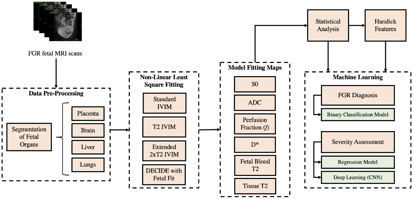
Model fitting techniques, described in Section 3.2, were applied to the segmented organs of interest, to yield quantitative parameters describing various signals. These parameters were then employed to perform texture analysis from multi-contrast MRI modelling, as described in Section 3.3. Results from the model fitting were used as inputs to the classifier and regressor in Sections 3.6 to 3.8 to predict a diagnosis of FGR and the GA at delivery. An overview of this pipeline is depicted in Figure 1.

3.1 Data
Patient MRI scans of voxel resolution 1.9x1.9x6 were acquired using the acquisition parameters from (Melbourne et al. (2019)), where b-values and echo times are varied in pairs (enabling both T relaxometry and DW-MRI fitting), using a 1.5 T Siemens Avanto and performed under free-breathing. The dataset consisted of 12 early-onset FGR (Gordijn et al. (2016a)) ranging between [24, 33] gestation weeks, and 12 control pregnancies with MR data ranged between [25, 34] GA interval, (Median 28wks3wks) respectively. Specific details on subject inclusion criteria are available in (Aughwane et al. (2020b)). The study was approved by the UK National Research Ethics Service and all participants gave written informed consent (REC reference 15/LO/1488).
There are biological mechanisms that may cause differences in the distribution of blood perfusion throughout the fetus in FGR. To investigate this, manual segmentation of the placenta, liver, lungs and brain was accomplished using the open-source ITK-SNAP application (image segmentation). The resultant 3D mask files were used within the NiftyFit package (Melbourne et al. (2016b)) for multi-parametric model-fitting (Melbourne et al. (2019)), and to perform texture analysis.
3.2 Model Fitting
Model fitting techniques were applied to each organ segmentation over the averaged region of interest (ROI) signal and on a voxelwise scale, yielding quantitative metrics for both approaches. Non-linear least squares were used to perform the fitting, with voxelwise fitting being initialised with the ROI parameter estimates - enhancing signal-to-noise ratio (SNR) by reducing the changes of fitting to local minima. A range of models were explored, including simple T and ADC estimation, as well as more complex models based on IVIM (Le Bihan et al. (1986)) and DECIDE (Melbourne et al. (2019)). Investigated in this research were parameters linked to diffusion, but they do not represent diffusion directly. The simplest T model fitting describes the MRI signal as
| (2) |
where are the echo times, is the measured signal, and the baseline signal. Regarding simple ADC fitting, this is accomplished using
| (3) |
where b are the b-values. Thus, the acquired data requires varying and b-values to allow for dual ADC and T2 model fitting.
The IVIM model describes perfusion as a pseudodiffusion process (represented by a pseudodiffusion coefficient, D), by characterising the collective motion of blood water molecules within the vessel network as a random walk. The IVIM model also incorporates “true” diffusion of water molecules (ADC), modelling the signal as
| (4) |
where is the perfusion fraction (volume occupied by incoherently flowing blood in a given voxel) and is the b-value (Le Bihan (2019)). We refer to this model as Standard IVIM (Eq. 4). This can be extended to incorporate T relaxometry as
| (5) |
We refer to this model (Eq. 5) as T2 IVIM. However, this model presents inherent limitations, as it assumes both vascular and tissue compartments (parametrised by pseudo-diffusion and true diffusion coefficients) have the same T value, leading to an overestimation of the pseudo-diffusion volume fraction with increasing echo time () (Jerome et al. (2016)). Thus, the presented analysis incorporates more complex models, accounting for varying blood and tissue T values:
| (6) |
with being the perfusion fraction, T and T being the transverse relaxation time for the pseudo-diffusion compartment (blood) and true diffusion compartment (tissue), respectively (Jerome et al. (2016)). We refer to this model as Extended T2 IVIM (Eq. 6).
The DECIDE model (Melbourne et al. (2019)) was also applied specifically to the placenta, which assumes three compartments with distinct diffusivity and relaxivity: fetal capillaries, trophoblast space and maternal blood pool. This model, given by Equation 7, enables computation of novel placental biomarkers including maternal fetal blood volume ratio and fetal blood saturation.
| (7) |
Here, T, T and T represent the transverse relaxation times for fetal blood, maternal blood and trophoblast space, respectively; and is the maternal blood volume fraction. R and R are fixed known, and respectively at 1.5T), taken from (Melbourne et al. (2019)).
3.3 Texture Analysis
The aim of texture analysis was to examine the spatial arrangement of intensities in the segmented organs using in-house software developed in MATLAB (The MathWorks Inc., Natick, MA). To perform the texture analysis, a grey level co-occurrence matrix (GLCM) was computed to provide insight into the spatial interaction of neighbouring pixels. Haralick features are statistical features extracted from the GLCM to describe the overall image texture using measures encompassing energy, entropy, correlation, contrast, variance, and homogeneity (Haralick et al. (1973)):
Energy: This measure is extracted from the angular second moment, which calculates the grey level local uniformity,
| (8) |
where and represent the image dimensions, and corresponds to an element of the normalised GLCM.
Entropy: A statistical measure of randomness.
| (9) |
Correlation: A measurement of the similarity between neighbouring pixels,
| (10) |
where ; are the means and ; are the standard deviations.
Contrast: The number of grey levels that exist in the scan.
| (11) |
Variance: A measure of variability.
| (12) |
Homogeneity: The number of changes of intensity that appear in a region of interest.
| (13) |
We hypothesised that these six Haralick features could be used to discern between FGR and appropriately grown fetuses due to a lower SNR present in FGR fetuses as a result of lower and decreased oxygen saturation (Portnoy et al. (2017)). We expected that the lower signal intensities in FGR compared to controls would be especially evident in the placenta and fetal liver and correlate directly with placental insufficiency (Aughwane et al. (2020a); Kessler et al. (2009)). For instance, this would be reflected in the computed Haralick features by observing lower contrast values in FGR fetuses in comparison to the controls. Decreased contrast in the ROI would equate to an increase in homogeneity.
These features were computed for each subject on the most significant parameter maps for each organ (as determined by the t-tests described in Section 3.4 with a p-value cut-off of 0.05), as well as the b=0 volume with lowest echo time from the original IVIM T-weighted MRI scan; this yielded interpretable texture descriptors (Haralick et al. (1973); Bharati et al. (2004)). The images were quantised into grey level bins of fixed equal width for between-subject texture feature value comparisons. Single-factor analysis of each feature was conducted between the FGR and control patients. Results from the texture analysis were then concatenated by considering the mean and max of each Haralick feature.
3.4 Feature Statistical Significance
The model fitting maps provide voxelwise information for each of the parameters optimised for. We simplified this information by considering the mean, max, variance and mode of each of voxelwise map. This yielded reduced parameters to be used for subsequent classical ML-based assessments.
We performed statistical analysis on these simplified model fitting parameters and on the Haralick features, in order to identify the most significant features in differentiating between the control and FGR cohorts. A Shapiro–Wilk test was used to confirm normality of the parameters obtained from the model fitting on a patient-by-patient basis to verify it was justifiable to run a t-test on them. In particular, the Shapiro-Wilk test was selected for its efficacy on small sample sizes. The test was run on the distribution of the model fitted parameters for each of the organ ROIs done over all of the samples split between the two cohorts.
T-tests were then carried out between the two cohorts for all the model fitted parameters, Haralick features, and organ ratio parameters. Results with p-value less than 0.05 indicated statistically significant differences between the control and FGR group means.
We used these significant parameters for training simple classical machine learning models on classification (control or FGR) and regression (GA at birth, time from scan until birth and baby weight), as detailed in the following sections.
3.5 FGR Biomarkers for Machine Learning Outcome Predictions
Following these statistical tests, we aimed to explore the use of these significant features (p-value in distinguishing between controls and FGR) as potential FGR biomarkers for severity assessments. For this, we conducted various ML training experiments, employing a binary classifier for diagnosis prediction (control or FGR), and simple regressors to predict GA at birth, time from scan until birth, and baby weight.
Our training experiments explored the most appropriate use of our data to achieve optimal results. For this, we trained each model first using exclusively model fitting data (mean, max, variance and mode of each of voxelwise map), followed by exclusive training using Haralick features, and finally combining both model fitting data and Haralick features. Only the features with a p-value in differentiating between controls and FGR cohorts were employed.
3.6 Binary Classification for FGR Diagnosis
We employed logistic regression for binary classification, using a stochastic average gradient (SGA) solver that supports the L1 regularisation to minimise the cross-entropy loss function.
This classifier models the conditional probability of an FGR or non-FGR (control) diagnosis, Y, given input features, X (model fitting data and Haralick features), by applying a sigmoid function to the output of a decision function , which ensures an output between 0 and 1:
| (14) |
where X is the input feature vector, and w is the learnt weight vector. These probability scores (i.e. the output for Eq. 14) are mapped to discrete classes with a decision boundary of 0.5, that is, an output probability indicates an FGR diagnosis, while an output probability specifies a non-FGR diagnosis.
The optimal regularisation parameters (found via a grid search) were an L1 ratio of 0, i.e. L2 regularisation for all classifiers; and a regularisation strength () of 0.001 for the classifier trained exclusively on model fitting features, as well as the joint model (Haralick and model fitting features), while the model trained only on Haralick features yielded a .
Based on RFECV, we used 44 out of 84 features for the classifier trained on model fitting data; 34 out of 53 features for the classifier trained on Haralick features; and 118 out of 137 for the classifier trained on both feature types.
3.7 Linear Regression Model for Severity Assessment
We trained three multi-variate linear regressors to predict GA at delivery, time interval between scan and delivery, and baby weight, as these variables () are potential indicators of FGR severity. Thus we fitted a linear equation to our feature matrix X, minimising the sum of squared errors between predicted and expected target values (including L1 and L2 regularisation) in order to find the weights, w.
Refer to Table 3 in Section 4.5 for information regarding model tuned hyperparameters and number of selected features for each regressor.
3.7.1 Training Split and Feature Selection
For our simple ML classifier and regressors, the data was split into 80% for training (n=18) and 20% for testing (n=5). The training set was used for hyperparameter tuning using 5-fold cross validation. The reduced sample size in our research was confronted by additionally employing our training set to obtain 5-fold cross validated evaluation metrics, as well as the final test set metrics.
Recursive feature elimination with 5-fold cross validation (RFECV) was implemented on the training set to determine the optimal number of features for each ML model.
3.8 Deep learning for Severity Assessment
The regression methods described in Section 3.7, use data which statistically shows differences between FGR and healthy (p-value0.05), followed by RFECV feature selection, to further reduce the noise present. However, the features used (in Section 3.7), particularly the model fitting features, drastically reduce the amount of parameter maps information: by taking single statistical values over whole voxelwise maps (i.e. mean, max, min, mode), important spatial relationships and detailed voxel-level information may be eliminated. The Haralick features do contain information regarding spatial arrangements and intensity relationships, which supports our previous method.
In an attempt to make use of this detailed information contained within each parameter map, we explored the potential of a Convolutional Neural Network (CNN) for severity assessment, aiming to predict the same regression variables as with our simple ML models (GA at birth, time interval from scan until delivery, and baby weight).
3.8.1 Data pre-processing
We used the voxelwise parameter maps for the liver and placenta only, as we found these organs to consistently have the highest number of significant differences between controls and FGR. We concatenated the first layer, the signal, of the volumetric image (i.e. the b=0 volume with the lowest echo time from the raw acquisition) with fitted parameter maps from the Extended T2 IVIM model for the liver (perfusion fraction , , T, T and ADC); and fitted parameter maps from the DECIDE model for the placenta (, , , T, T, ADC), yielding a total of twelve input channels.
The maps we selected were only those pertaining to the models which give us most information, which are the most complex models. Higher complexity models are more prone to add noise to the fitted maps. Contrasting to this, our input to the simple linear regressors were highly processed and selected features: we first took various extremely simplifying metrics of our voxelwise map (e.g. taking the mean), followed by selecting only those that present a statistical significance between both cohorts, in addition to RFECV. This provides us with features which are highly representative of distinctions between controls and FGR groups.
The data was split into 80% for training (N=18), and 20% for testing (N=5). The intensity of all images were normalised by subtracting the mean and dividing by the standard deviation, followed by scaling between 0 and 1. We used Gaussian noise, intensity shifts, bias field, contrast adjustments, axis flips, and affine deformations for data augmentation.
3.8.2 CNN implementation details
A five layer residual neural network (ResNet) (He et al. (2016)) was employed for each of our regression predictions, with output channels = [64, 64, 128, 256, 512], with respective strides = [1, 1, 2, 2, 2], applying two 3D convolutions for each residual block (kernel size of 3). Instance normalisation (Ulyanov et al. (2016)) was used after each convolution, followed by Parametric Rectified Linear Unit (PReLU) activation functions (He et al. (2015)).
Mean Squared Error (MSE) was leveraged as the loss function, with an AdamW optimiser. A weight decay of was employed for all of our regression networks, with a learning rate (LR) = for predicting baby weight; and LR = for predicting GA at birth and time from MRI scan to delivery.
4 Results
4.1 Model Fitting
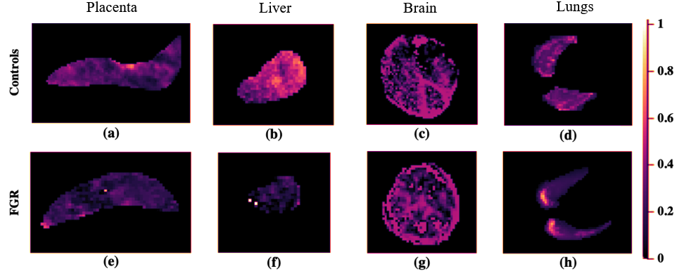
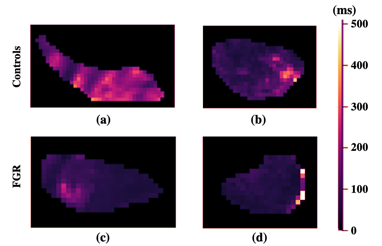
Figure 2 depicts examples of the parameter maps obtained from the model fitting techniques. The lower parameter map intensities in FGR compared to that in the controls is indicative of hypoperfusion and low oxygen saturation levels in these fetal organs. The T maps display pronounced differences in the signal intensities of both cohorts.
The most significant parameters in identifying differences between controls and FGR fetuses were the perfusion fraction, S, pseudo-diffusion coefficient (D), and T as given in Table 1. The placenta and liver were determined to be the most influential organs in diagnosing FGR.
The results for the parameter feature importances in Table 1, specify that there were no significant differences detectable in the fetal brain and lungs between normal and FGR fetuses, especially compared to the placenta and liver, where differences were significant.
| Model Fitting Technique | Parameter | Average Metric | Pairwise Group Comparison | Organ | T Statistic | P-Value |
|---|---|---|---|---|---|---|
Dependent IVIM | D* | Mean | Control vs FGR | Placenta | -4.597300242 | 0.00015589 |
Extended 2xT2 Dependent IVIM | D* | Mean | Control vs FGR | Placenta | -4.560436097 | 0.000170214 |
DECIDE Model (Voxelwise Measurements) | D* | Mean | Control vs FGR | Placenta | -4.205788361 | 0.00039723 |
Extended 2xT2 Dependent IVIM | Perfusion Fraction | Min | Control vs FGR | Placenta | 3.725183003 | 0.001250966 |
Extended 2xT2 Dependent IVIM | Perfusion Fraction | Mode | Control vs FGR | Placenta | 3.725183003 | 0.001250966 |
Standard IVIM | Perfusion Fraction | Median | Control vs FGR | Liver | 3.624757118 | 0.001587669 |
T2 Dependent IVIM | T2 | Min | Control vs FGR | Placenta | 3.463092031 | 0.002326109 |
Extended 2xT2 Dependent IVIM | Perfusion Fraction | Median | Control vs FGR | Placenta | 3.27041186 | 0.003653498 |
T2 Dependent IVIM | Perfusion Fraction | Min | Control vs FGR | Placenta | 3.249455242 | 0.003836258 |
T2 Dependent IVIM | Perfusion Fraction | Mode | Control vs FGR | Placenta | 3.249455242 | 0.003836258 |
4.2 Texture Analysis
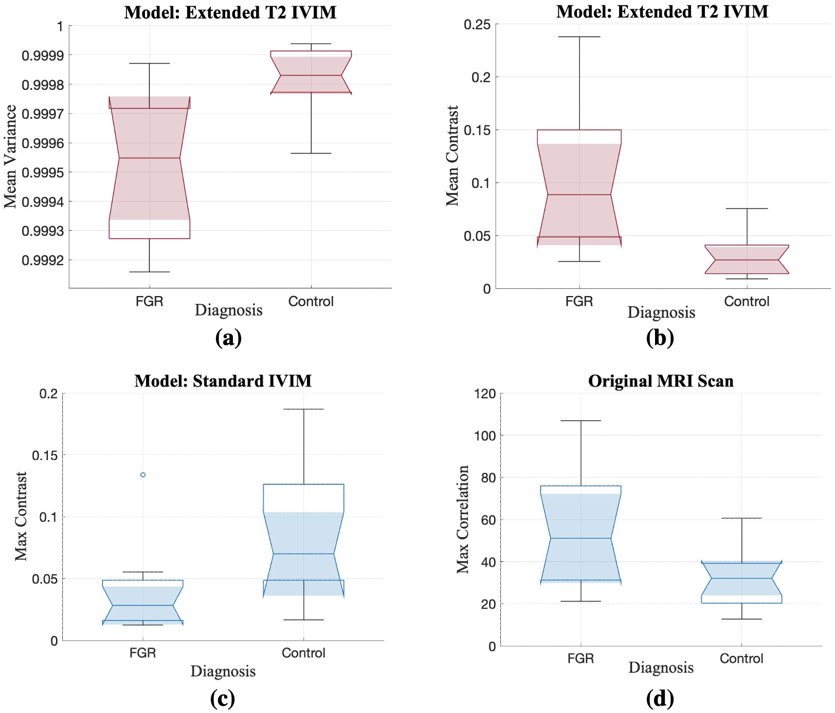
Evaluation of the resulting Haralick features corroborated the degree of effect on the placenta in FGR, particularly using the Extended T IVIM map and its mean variance. The brain was the least significantly different organ in this analysis. Greater mean variance in the signal from the Extended T IVIM model of the healthy cohort (refer to Figure 4(a)), is indicative of increased heterogeneity in FGR placentas. The max correlation of the liver perfusion fraction in the controls in Figure 4(d) reflects larger intensity differences compared to FGR. This is a significant feature to consider in the Standard IVIM model when studying the liver in FGR, especially given that the notches do not overlap between the cohorts.
4.3 FGR Diagnosis via a Classification Model
| Training Dataset | Cross Validation (N = 18) | Testing (N = 5) | RFE | ||
|---|---|---|---|---|---|
| Accuracy | Accuracy | Sensitivity | Specificity | Top Five Features (Model) | |
| Model Fitting Features | 95 ± 10% | 100% | 100% | 100% | Placenta mean D* (T2 IVIM) |
Placenta mean D* (Extended 2xT2 IVIM) | |||||
Placenta mean D* (DECIDE) | |||||
Liver/Lungs median perfusion fraction (Standard IVIM) | |||||
Placenta/Lungs median perfusion fraction (Extended 2xT2 IVIM) | |||||
| Haralick Features | 77 ± 12% | 80% | 67% | 100% | Placenta mean variance D* (Extended 2xT2 IVIM) |
Placenta max correlation D* (Extended 2xT2 IVIM) | |||||
Placenta mean correlation D* (T2 IVIM) | |||||
Liver max contrast D* (Standard IVIM) | |||||
Liver mean contrast D* (Standard IVIM) | |||||
| Combined Features | 88 ± 15% | 100% | 100% | 100% | Placenta mean D* (T2 IVIM) |
Placenta mean D* (Extended 2xT2 IVIM) | |||||
Placenta mean D* (DECIDE) | |||||
Liver/Lungs median perfusion fraction (Standard IVIM) | |||||
Placenta/Lungs median perfusion fraction (Extended 2xT2 IVIM) | |||||
Referring to the results presented in Table 2, the classifier performs best when trained exclusively on model fitting data, achieving a prediction accuracy of 100% in testing, and thus a precision and recall score of 1.0.
This is further validated by the cross validated accuracy on training set, with a standard deviation of only 10% across folds, hinting at optimal model generalisability.
4.4 Classification Feature Importance
Given our optimal test set classification results (see Table 2), we qualitatively assess the most important features driving each classifier model. These were obtained via Recursive Feature Elimination (RFE). We obtained the exact same top five features for both the logistic regressor trained exclusively on model fitting data, and the logistic regressor trained on both Haralick features and model fitting data.
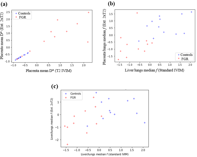
Figure 5b shows distinct differences between controls and FGR cohorts. Here, control subjects display a much higher placenta and liver perfusion relative to the lungs, compared to FGR subjects. This is an indicator that in FGR, both the placenta and the lungs are much less perfused than other vital organs such as the lungs.
The differences between the performance of the model fitting techniques can be inferred from Figure 5c. It showcases the ‘liver/lungs median f’ plotting the Extended 2xT2 IVIM model against the Standard IVIM model. When projected onto each axis, the x-axis (i.e. the Standard IVIM model), permits a more accurate linear classification between the cohort compared to the Extended 2xT2 IVIM model. Seemingly, the Standard IVIM model produces a better fit to our data (for this particular parameter) than the more complex models with additional parameters, potentially due to the noise present.
4.5 Severity Assessment via a Regression Model
| Prediction | TrainingDataset | Regularisationstrength () | RegularisationRatio (L1/L2) | RFECV(SelectedFeatures/TotalFeatures) | Cross Validation (N = 18) | Testing (N = 5) |
| RMSE ± STDEV | RMSE | |||||
| GA at[] Delivery | Model Fitting Features | 33.93 | L2 only | 71/84 | 2.9 ± 2.36 weeks | 2.1 weeks |
Haralick Features | 0.49 | L1 only | 5/53 | 4.48 ± 4.13 weeks | 3.06 weeks | |
Combined Features | 44.98 | L2 only | 119/137 | 3.0 ± 2.42 weeks | 3.1 weeks | |
| Time from[] scan until[] delivery | Model Fitting Features | 59.64 | L2 only | 84/84 | 3.21 ± 2.53 weeks | 3.12 weeks |
Haralick Features | 1.15 | L1 only | 5/53 | 4.95 ± 3.51 weeks | 4.82 weeks | |
Combined Features | 7.20x10 | 0.31 | 133/137 | 3.5 ± 2.68 weeks | 3.09 weeks | |
| Baby weight | Model Fitting Features | 2.32x10 | 0.16 | 64/84 | 372.71 ± 334.42 g | 991.36 g |
Haralick Features | 25.6 | 0.92 | 28/53 | 738.88 ± 600.58 g | 1591.72 g | |
Combined Features | 3.56 | L1 only | 5/137 | 668.64 ± 488.42 g | 1099.06 g |
Table 3 includes our test set and cross validated regressor results. In accordance with our classifier results, the models with highest performance are those trained on model fitting features, excepting predictions for time from scan until delivery, where the combined model displays an insignificantly lower root mean square error (RMSE) on test set compared to the model trained exclusively on model fitting data.
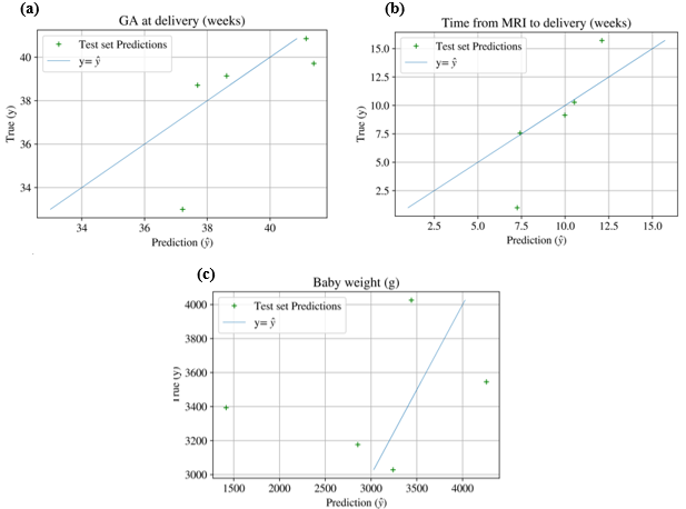
Figure 6 depicts test set regression predictions for our best performing regressors, against true labels. Qualitatively, the test set predictions that mostly resemble the true data points are from the time interval between MRI and delivery (Figure 6b), however this has two important outliers. It is complex to comment on the significance of this, given the extremely small test set. The plot depicting baby weight predictions (Figure 6c) visually appears as the worst fit, however the value range for this variable is much larger, which may partially explain this. Additionally, the most important outliers for baby weight are predictions which are lower than the actual baby weight, which is clinically significant: it is best to overestimate the severity than underestimate it.
4.6 Deep Learning Regression
| RMSE on Test Set (N = 5) | ||
|---|---|---|
| GA at delivery | Time from scan until delivery | Baby weight |
| 5.33 weeks | 5.93 weeks | 1169.88 g |
5 Discussion
In this study, we combined model fitting techniques, texture analysis from multi-contrast MRI modelling, and ML models, to facilitate multi-fetal organ analysis of FGR. This provided a more holistic approach to imaging this common pregnancy condition and presented an approach towards automated diagnosis and severity assessment. Differences between FGR and non-FGR fetuses were observed, particularly in the placenta and fetal liver, emphasising the significant effect of FGR on these organs.
Overall, the fitted model parameters reveal decreased f, T, and D in the liver and placenta in FGR fetuses compared to the controls. These findings are validated by those from (Shi et al. (2019); Siauve et al. (2019); Razek et al. (2019); Aughwane et al. (2021)). The hierarchy of feature importances in Table 1 suggests that the brain and lungs may benefit from alternative analysis, focusing on certain cortical regions for the brain, and incorporating alternative imaging modalities for the lungs, as model fitting MRI analysis may not be the most appropriate technique for this fluid-filled organ. These differences are indicative of a reduced oxygen saturation and perfusion within these organs, as well as abnormal capillary blood flow motion (Aughwane et al. (2020b)). We did not observe significant differences in the properties of fetal brains and lungs between the FGR and control groups.
The most influential Haralick features were extracted from the perfusion fraction measurements, particularly computed from the Extended T IVIM and Standard IVIM models. Another important parameter determined by the Haralick features was T, attributed to its correlation with oxygen saturation (lower T reflects a lower oxygen saturation (Portnoy et al. (2017))).
The placenta was established as the organ with most significant textural differences between the FGR and control groups. Variance, contrast, entropy and energy in placental perfusion fraction maps were the most significant textural differences between FGR and controls. This may be related to differences in the presence of maternal and fetal vascular malformation (Mifsud and Sebire (2014a); Burton et al. (2009)).
The second organ with greatest textural differences between both cohorts was the liver, particularly the D maps (contrast, correlation, and energy), indicating spatial differences in the incoherent fetal capillary blood motion in this organ. This may indicate an abnormal blood motion in the liver compared to a healthy developing organ, affecting nutrient supply to this organ and may be related to the role of the ductus venosus in redistributing blood to the heart under the influence of increasing hypoxia (Mifsud and Sebire (2014b)). Energy was heavily influenced by the number of grey levels and was, therefore, a significant feature for the placenta, lungs and brain, due to the presence of similar intensity voxels within local regions. Correlation was affected by the noise present in the image, which explains the notable correlation differences found in the liver, being the organ with the lowest SNR.
The feature importances determined by RFE for the classifier in Section 4.4, and the fact that they coincide with the top five features for the logistic regressor, indicate that these are very strong features in determining model predictions. The top five features from our best regressor models are those involving the liver f, placenta f, placenta D*, placenta tissue T2, and liver/lung D*. Thus, the top features we obtained here are very similar to those from our binary classifiers, which strengthens our argument that the liver and placenta may be less well perfused in FGR, with altered circulation patterns. We additionally found placental tissue T2 as a significant feature for severity predictions. Tissue T2 is related to tissue oxygenation. Therefore, the fact that this is one of our most important features for severity assessment may be linked to reduced placental oxygenation in more severe cases, affecting fetal growth.
In particular, these features all involve either the placenta and the liver, which supports our prior t-tests and Haralick feature analysis. Two markedly informative features are the ratios of Placenta/Lungs and Liver/Lungs median perfusion fractions (f). These features suggest that in control subjects, the relative perfusion of the liver and placenta compared to the lungs is much higher than in FGR cases, i.e. the liver and placenta are not deprived of nutrients, as may be the case in FGR.
The recurrence of the D* and in the top features demonstrate these may be potential FGR biomarkers. Figure 5 includes a visual depiction of the mean D*, as computed from two different models. The linear relationship between variables on the leftmost plot (a) is due to the axis representing the same variable, as computed from two different models, thus differences are due to different model assumptions and noise. This plot clearly show abnormal D* placenta values for FGR subjects, with these displaying a much larger spread compared to controls. This pseudo-diffusion coefficient (D*) describes macroscopic intra-capillary blood motion. Thus, these results are suggestive of abnormal placental circulatory patterns, which may be due to placental insufficiencies and dysfunctions in FGR.
While blood in the intervillous space appears to undergo incoherent motion, the maternal blood fraction is not attributed to D* in addition to ADC in Equation 7, as previously modelled by (Melbourne et al. (2019)). Our working assumption within the modelling is that maternal blood arrives at high-flow, low-velocity, resulting in an overall lower D* value compared to that for fetal intra-capillary blood and moves slowly through the villous structure. It is probable that this assumption is less true close to the spiral artery inlets - but this remains to be fully validated.
Placental and liver perfusion fraction, D* and tissue T2 were amongst the most important features for our ML binary classifiers and linear regressors, as determined by RFE. This supports our choice of most important textural differences and aforementioned biological reasoning. The classifier achieved 100 accuracy on the test set, indicating that the model features are powerful indicators for FGR detection. But these results require prospective validation in a larger study population due to the small test group size (n=5) in this proof-of-concept study, which may have resulted in overfitting of the models to the features. Moreover, a larger dataset would permit the transition into more complex prediction models in future research.
The RMSE of 2.1 weeks and 3.09 weeks for our linear regressor predicting GA at delivery and time interval from scan until delivery, respectively, encode a large window in terms of fetal development. Recent research conducted by Yamauchi et al. employed leave-one-out cross validation to predict GA in normal and complicated pregnancies from urinary metabolite information (Yamauchi et al. (2021)). The authors achieved a Pearson correlation coefficient of 0.86 between the true and predicted GAs during normal pregnancy progression, and an RMSE of 26.7 gestation days (3.81 weeks). Thus, the performance of our regressor appears to be comparable with that from a model trained on 187 healthy pregnant women.
The results in Table 3 indicate a lower RMSE from the combined model compare to the model trained exclusively on model fitting data. This signifies that our model fitting maps have a higher difference in intensity values, rather than textural or spatial relationships, between control and FGR cohorts, and for varying degrees of condition severity. From a mathematical point of view, considering that our data presents a range of 3864 g for baby weight, 15 weeks for GA at birth and 15.57 weeks for time interval between MRI scan and delivery; our RMSE on test set only represent 25%, 19.85% and 14% out of our total dataset range for baby weight, scan to birth interval, and GA at birth, respectively.
However, from a clinical perspective, offering a prediction with a RMSE of 2-3 weeks may not be of much added clinical value, given the close monitoring of FGR pregnancies, particularly in the weeks leading up to birth. These clinical patient management schemes offer a much tighter range of potential and optimal delivery dates. Nonetheless, the purpose of our regressors is not to supplant current delivery prognosis practices, but to aid in providing tailored patient assessments of severity, maximising information extracted from MRI scans, not currently considered routine clinical practice (i.e. model fitting techniques and organ comparison assessments).
From this, we demonstrate the ability of our method to provide insights into how fetal organs are affected in FGR, using this information to establish optimal delivery time within a two week range, which in future work may be of use to establish which pregnancies must be closely monitored. While we expect more severe cases to require early delivery, we do make important assumptions for these predictions, namely that all cases were delivered using the exact same criteria (when in practice patient view may also have influenced delivery choices), and that the appropriate and optimal clinical decisions were made, which is not unreasonable considering all our cases are from a specialised FGR unit.
For this reason, we also investigated baby weight as a postnatal severity metric. We obtained optimal results for this metric, which demonstrates that fetal organ features such as perfusion are closely related to appropriate fetal growth, as determined by postnatal weight.
The ResNet prediction results in Table 4 concluded a much higher RMSE compared to our simpler logistic regression model. There are many potential reasons for this, such as the amount of noise in our CNN input data. Another evident reason for our poorer deep learning results is our small sample size, which, although we employed augmentation techniques, may still be insufficient to reliable train a CNN. Nonetheless, we obtained much closer results to our linear regressors for baby weight ResNet predictions. The fact that we included MRI scan data as our first channel may play a role in this, as baby weight is closely related to fetal size, which may be assessed from this first channel. Another factor to consider is the 6mm slice thickness of the scans being of a comparable size to the fetal organs. The structures of interest, such as the signal intensities of small vascular features and smaller tissue compartments (for instance in the fetal kidney), may have been susceptible to partial volume averaging compared to the brain, which is a bigger structure in comparison. However, our multi-compartment modelling takes this effect into account to some degree by attributing the signal from a single large voxel to different tissues.
Our deep learning method demonstrates how our organ model fitting maps contain spatial and intensity information which may be efficiently retrievable via CNNs, and presents potential to aid in providing condition information. Future work could test this directly with the current dataset by skipping the model fitting step. But there would be a resulting trade-off between interpretation (from validated MRI physiological models) and clinical predictivity (where ML techniques are a relative black-box for accurate prediction in absence of interpretability).
Our method proposed in this preliminary evaluation must be refined before translation to a clinical environment, but it may serve as a guide on condition severity. In practice though, this tool would also be used in conjunction with a wide range of information and existing biomarkers, including ultrasound data on fetal size, and maternal and fetal Doppler analysis of vascular resistance, which we have not included so far in this work. The ML analysis on these results supports the potential use of these parametric biomarkers in measuring FGR and providing an estimate of severity, including an indication of the likely GA at delivery. In addition to these biomarkers, future work could systematically include volumetric data on the brain, lungs, liver, and placenta to better enhance the ML models. However, the data was unregistered, did not use 3D reconstruction and would require direct comparisons to pre-published normative curves to know how lung/organ volume changes with gestation to incorporate fully. It is also important to note that the method employed assumes the delivery time of each subject was optimal, which although extracted from an early-onset clinic with specialised treatment, this may not be always the case, inducing biases.
The deep learning extension implemented to target this regression problem showcases potential avenues for future work with this type of voxelwise organ model fitted maps. These maps contain important spatial information, which proved useful to assess postnatal baby weight. Future work on deep learning should focus on appropriately selecting the input channel features, by conducting detailed assessments on the level of noise against information quality and significance.
Analysis on parameter correlations indicated that as the perfusion fraction in the liver and placenta decreased, the more severely growth-restricted the FGR fetuses were. This corroborated our initial hypotheses for selecting the fetal liver and placenta as severely-affected organs in FGR, with SNR perhaps too low and variability too high to observe differences in the fetal brain and lung. However, further work is needed to refine the analysis of the signals from these organs to better study the impact of FGR.
Moreover, reliance of ML models on ‘Big Data’ (Wang and Alexander (2016)), motivates the need for a larger dataset, or data augmentation techniques to improve model performance and reduce generalisation error. Increased data availability could enable deep learning models, such as CNNs, which show potential for large-scale diagnosis improvement (Yadav and Jadhav (2019)), compared to traditional ML models. Our dataset of 24 subjects limits the results and conclusions from being generalised to the population. But this was not the purpose of the study. Rather, we sought to investigate the concepts and statistical methods employed in this paper. Future work could extend the methods to additional pregnancy complications to diagnose not only, FGR and non-FGR, but also the presence of other pregnancy conditions.
6 Conclusion
In this proof-of-concept we proposed an approach to automate diagnosis of FGR using parameters extracted from the fetal liver and placenta, supported by the application of texture analysis. This preliminary investigation has demonstrated the potential of the models in assessing vascular properties of highly-perfused fetal organs, determined by multi-compartmental model fitting techniques. The placenta and fetal liver were prominent organs in identifying FGR fetuses, with key parametric features indicating a reduced perfusion, oxygenation and fetal capillary blood motion in these organs.
Our results prove that applying IVIM-based models on organs segmented from MRI scans generates features which are descriptive of FGR, i.e. potential biomarkers, enabling to construct simple machine learning models to predict diagnosis and offer insights into severity of the condition. The detailed voxel-level nature of our maps additionally enables deep learning experiments for condition severity assessments.
We validated our methodology on twenty-three FGR and control cases, achieving particularly optimal results for diagnosis classification. Our research exemplifies how ML models can be incorporated into the diagnostic workflow, as well as its potential to indicate severity of the condition. Future work into multi-organ fetal analysis will extend these techniques to other placental complications into a larger-scale study, using more complex ML and deep learning models.
Acknowledgments
This research was supported by the Wellcome Trust (210182/Z/18/Z, 101957/Z/13/Z, 203148/Z/16/Z and Wellcome Trust/EPSRC NS/A000027/1) and the Radiological Research Trust. The funders had no direction in the study design, data collection, data analysis, manuscript preparation or publication decision. We would like to thank Dr Magda Sokolska and Dr David Atkinson for their invaluable support and advice for the data collection in this work.
Ethical Standards
The work follows appropriate ethical standards in conducting research and writing the manuscript, following all applicable laws and regulations regarding treatment of animals or human subjects.
Conflicts of Interest
We have no conflicts of interest to report.
References
- Arabi Belaghi et al. (2021) Reza Arabi Belaghi, Joseph Beyene, and Sarah D McDonald. Prediction of preterm birth in nulliparous women using logistic regression and machine learning. PloS one, 16(6):e0252025, 2021.
- Arthurs et al. (2017) OJ Arthurs, A Rega, F Guimiot, N Belarbi, J Rosenblatt, V Biran, M Elmaleh, G Sebag, and M Alison. Diffusion-weighted magnetic resonance imaging of the fetal brain in intrauterine growth restriction. Ultrasound in Obstetrics & Gynecology, 50(1):79–87, 2017.
- Audette and Kingdom (2018) Melanie C Audette and John C Kingdom. Screening for fetal growth restriction and placental insufficiency. In Seminars in Fetal and Neonatal Medicine, volume 23, pages 119–125. Elsevier, 2018.
- Aughwane et al. (2020a) Rosalind Aughwane, Emma Ingram, Edward D Johnstone, Laurent J Salomon, Anna L David, and Andrew Melbourne. Placental mri and its application to fetal intervention. Prenatal diagnosis, 40(1):38–48, 2020a.
- Aughwane et al. (2020b) Rosalind Aughwane, Nada Mufti, Dimitra Flouri, Kasia Maksym, Rebecca Spencer, Magdalena Sokolska, Giles Kendall, David Atkinson, Alan Bainbridge, Jan Deprest, Tom Vercauteren, Sebastien Ourselin, Anna David, and Andrew Melbourne. MRI Measurement of Placental Perfusion and Oxygen Saturation in Early Onset Fetal Growth Restriction. BJOG: An International Journal of Obstetrics & Gynaecology, pages 1471–0528.16387, Jun 2020b. ISSN 1471-0528. doi: 10.1111/1471-0528.16387. URL https://onlinelibrary.wiley.com/doi/abs/10.1111/1471-0528.16387.
- Aughwane et al. (2021) Rosalind Aughwane, Nada Mufti, Dimitra Flouri, Kasia Maksym, Rebecca Spencer, Magdalena Sokolska, Giles Kendall, David Atkinson, Alan Bainbridge, Jan Deprest, et al. Magnetic resonance imaging measurement of placental perfusion and oxygen saturation in early-onset fetal growth restriction. BJOG: An International Journal of Obstetrics & Gynaecology, 128(2):337–345, 2021.
- Bengio (2012) Yoshua Bengio. Deep learning of representations for unsupervised and transfer learning. In Proceedings of ICML workshop on unsupervised and transfer learning, pages 17–36. JMLR Workshop and Conference Proceedings, 2012.
- Beune et al. (2018) Irene M Beune, Frank H Bloomfield, Wessel Ganzevoort, Nicholas D Embleton, Paul J Rozance, Aleid G van Wassenaer-Leemhuis, Klaske Wynia, and Sanne J Gordijn. Consensus based definition of growth restriction in the newborn. The Journal of pediatrics, 196:71–76, 2018.
- Bharati et al. (2004) Manish H Bharati, J Jay Liu, and John F MacGregor. Image texture analysis: methods and comparisons. Chemometrics and intelligent laboratory systems, 72(1):57–71, 2004.
- Burgos-Artizzu et al. (2020) Xavier P Burgos-Artizzu, David Coronado-Gutiérrez, Brenda Valenzuela-Alcaraz, Elisenda Bonet-Carne, Elisenda Eixarch, Fatima Crispi, and Eduard Gratacós. Evaluation of deep convolutional neural networks for automatic classification of common maternal fetal ultrasound planes. Scientific Reports, 10(1):1–12, 2020.
- Burton et al. (2009) Graham J Burton, Andrew. W Woods, Eric Jauniaux, and John CP Kingdom. Rheological and Physiological Consequences of Conversion of the Maternal Spiral Arteries for Uteroplacental Blood Flow during Human Pregnancy. Placenta, 2009. ISSN 01434004. doi: 10.1016/j.placenta.2009.02.009.
- Caly et al. (2021) Hugues Caly, Hamed Rabiei, Perrine Coste-Mazeau, Sebastien Hantz, Sophie Alain, Jean-Luc Eyraud, Thierry Chianea, Catherine Caly, David Makowski, Nouchine Hadjikhani, et al. Machine learning analysis of pregnancy data enables early identification of a subpopulation of newborns with asd. Scientific reports, 11(1):1–14, 2021.
- Chalouhi and Salomon (2014) GE Chalouhi and LJ Salomon. Bold-mri to explore the oxygenation of fetal organs and of the placenta. BJOG: An International Journal of Obstetrics & Gynaecology, 121(13):1595–1595, 2014.
- Chang et al. (2006) Chiung-Hsin Chang, Chen-Hsiang Yu, Huei-Chen Ko, Chu-Ling Chen, and Fong-Ming Chang. Predicting fetal growth restriction with liver volume by three-dimensional ultrasound: efficacy evaluation. Ultrasound in medicine & biology, 32(1):13–17, 2006.
- Colella et al. (2018) Marina Colella, Alice Frérot, Aline Rideau Batista Novais, and Olivier Baud. Neonatal and Long-Term Consequences of Fetal Growth Restriction. Current Pediatric Reviews, 14(4):212–218, Jul 2018. ISSN 15733963. doi: 10.2174/1573396314666180712114531.
- Couper et al. (2020) Sophie Couper, Alys Clark, John M D Thompson, Dimitra Flouri, Rosalind Aughwane, Anna L David, Andrew Melbourne, Ali Mirjalili, and Peter R Stone. The effects of maternal position, in late gestation pregnancy, on placental blood flow and oxygenation: An MRI study. The Journal of Physiology, 2020. ISSN 0022-3751. doi: 10.1113/jp280569.
- Crockart et al. (2021) IC Crockart, LT Brink, C du Plessis, and HJ Odendaal. Classification of intrauterine growth restriction at 34–38 weeks gestation with machine learning models. Informatics in medicine unlocked, 23:100533, 2021.
- Derwig et al. (2013) Iris Derwig, GJ Barker, Leona Poon, Fernando Zelaya, P Gowland, DJ Lythgoe, and Kypros Nicolaides. Association of placental t2 relaxation times and uterine artery doppler ultrasound measures of placental blood flow. Placenta, 34(6):474–479, 2013.
- Dundar et al. (2008) M Murat Dundar, Glenn Fung, Balaji Krishnapuram, and R Bharat Rao. Multiple-instance learning algorithms for computer-aided detection. IEEE Transactions on Biomedical Engineering, 55(3):1015–1021, 2008.
- Ebbing et al. (2009) Cathrine Ebbing, Svein Rasmussen, Keith M Godfrey, Mark A Hanson, and Torvid Kiserud. Redistribution pattern of fetal liver circulation in intrauterine growth restriction. Acta obstetricia et gynecologica Scandinavica, 88(10):1118–1123, 2009.
- Erickson et al. (2017) Bradley J Erickson, Panagiotis Korfiatis, Zeynettin Akkus, and Timothy L Kline. Machine learning for medical imaging. Radiographics, 37(2):505–515, 2017.
- Frias et al. (2015) Antonio E Frias, Matthias C Schabel, Victoria HJ Roberts, Alina Tudorica, Peta L Grigsby, Karen Y Oh, and Christopher D Kroenke. Using dynamic contrast-enhanced mri to quantitatively characterize maternal vascular organization in the primate placenta. Magnetic resonance in medicine, 73(4):1570–1578, 2015.
- Gardosi et al. (2013) Jason Gardosi, Vichithranie Madurasinghe, Mandy Williams, Asad Malik, and André Francis. Maternal and fetal risk factors for stillbirth: Population based study. BMJ (Online), 346(7893), Feb 2013. ISSN 17561833. doi: 10.1136/bmj.f108. URL http://www.bmj.com/content/346/bmj.f108?tab=related#webextra.
- Giger (2018) Maryellen L Giger. Machine learning in medical imaging. Journal of the American College of Radiology, 15(3):512–520, 2018.
- Gordijn et al. (2016a) S. J. Gordijn, I. M. Beune, B. Thilaganathan, A. Papageorghiou, A. A. Baschat, P. N. Baker, R. M. Silver, K. Wynia, and W. Ganzevoort. Consensus definition of fetal growth restriction: a Delphi procedure. Ultrasound in obstetrics & gynecology : the official journal of the International Society of Ultrasound in Obstetrics and Gynecology, 2016a. ISSN 14690705. doi: 10.1002/uog.15884.
- Gordijn et al. (2018) Sanne Jehanne Gordijn, Irene Maria Beune, and Wessel Ganzevoort. Building consensus and standards in fetal growth restriction studies. Best Practice & Research Clinical Obstetrics & Gynaecology, 49:117–126, 2018.
- Gordijn et al. (2016b) SJ Gordijn, IM Beune, B Thilaganathan, A Papageorghiou, AA Baschat, PN Baker, RM Silver, K Wynia, and W Ganzevoort. Consensus definition of fetal growth restriction: a delphi procedure. Ultrasound in Obstetrics & Gynecology, 48(3):333–339, 2016b.
- Haralick et al. (1973) Robert M Haralick, Karthikeyan Shanmugam, and Its’ Hak Dinstein. Textural features for image classification. IEEE Transactions on systems, man, and cybernetics, 1(6):610–621, 1973.
- He et al. (2015) Kaiming He, Xiangyu Zhang, Shaoqing Ren, and Jian Sun. Delving deep into rectifiers: Surpassing human-level performance on imagenet classification. In Proceedings of the IEEE international conference on computer vision, pages 1026–1034, 2015.
- He et al. (2016) Kaiming He, Xiangyu Zhang, Shaoqing Ren, and Jian Sun. Deep residual learning for image recognition. In Proceedings of the IEEE conference on computer vision and pattern recognition, pages 770–778, 2016.
- Hutter et al. (2019) Jana Hutter, Paddy J Slator, Laurence Jackson, Ana Dos Santos Gomes, Alison Ho, Lisa Story, Jonathan O’Muircheartaigh, Rui PAG Teixeira, Lucy C Chappell, Daniel C Alexander, et al. Multi-modal functional mri to explore placental function over gestation. Magnetic resonance in medicine, 81(2):1191–1204, 2019.
- Ingram et al. (2018) Emma Ingram, Josephine Naish, David M Morris, Jenny Myers, and Edward D Johnstone. 53: Mri measurements of abnormal placental oxygenation in pregnancies complicated by fgr. American Journal of Obstetrics & Gynecology, 218(1):S40–S41, 2018.
- Jacquier and Salomon (2021) M Jacquier and LJ Salomon. Multi-compartment mri as a promising tool for measurement of placental perfusion and oxygenation in early-onset fetal growth restriction. BJOG: An International Journal of Obstetrics & Gynaecology, 128(2):346–346, 2021.
- Jerome et al. (2016) Neil P Jerome, JA d’Arcy, T Feiweier, DM Koh, MO Leach, DJ Collins, and MR Orton. Extended t2-ivim model for correction of te dependence of pseudo-diffusion volume fraction in clinical diffusion-weighted magnetic resonance imaging. Physics in Medicine & Biology, 61(24):N667, 2016.
- Jiang et al. (2013) Lan Jiang, Paul T Weatherall, Roderick W McColl, Debu Tripathy, and Ralph P Mason. Blood oxygenation level-dependent (bold) contrast magnetic resonance imaging (mri) for prediction of breast cancer chemotherapy response: a pilot study. Journal of Magnetic Resonance Imaging, 37(5):1083–1092, 2013.
- Kessler et al. (2009) Jörg Kessler, Svein Rasmussen, Keith Godfrey, Mark Hanson, and Torvid Kiserud. Fetal growth restriction is associated with prioritization of umbilical blood flow to the left hepatic lobe at the expense of the right lobe. Pediatric research, 66(1):113–117, 2009.
- Khatibi et al. (2021) Toktam Khatibi, Elham Hanifi, Mohammad Mehdi Sepehri, and Leila Allahqoli. Proposing a machine-learning based method to predict stillbirth before and during delivery and ranking the features: nationwide retrospective cross-sectional study. BMC pregnancy and childbirth, 21(1):1–17, 2021.
- Kim et al. (2017) Daeun Kim, Eamon K Doyle, Jessica L Wisnowski, Joong Hee Kim, and Justin P Haldar. Diffusion-relaxation correlation spectroscopic imaging: a multidimensional approach for probing microstructure. Magnetic resonance in medicine, 78(6):2236–2249, 2017.
- Koivu and Sairanen (2020) Aki Koivu and Mikko Sairanen. Predicting risk of stillbirth and preterm pregnancies with machine learning. Health information science and systems, 8(1):1–12, 2020.
- Le Bihan (2019) Denis Le Bihan. What can we see with ivim mri? Neuroimage, 187:56–67, 2019.
- Le Bihan et al. (1986) Denis Le Bihan, Eric Breton, Denis Lallemand, Philippe Grenier, Emmanuel Cabanis, and Maurice Laval-Jeantet. Mr imaging of intravoxel incoherent motions: application to diffusion and perfusion in neurologic disorders. Radiology, 161(2):401–407, 1986.
- Lyall et al. (2013) Fiona Lyall, Stephen C Robson, and Judith N Bulmer. Spiral artery remodeling and trophoblast invasion in preeclampsia and fetal growth restriction: relationship to clinical outcome. Hypertension, 62(6):1046–1054, 2013.
- Malhotra et al. (2017) Atul Malhotra, Michael Ditchfield, Michael C Fahey, Margie Castillo-Melendez, Beth J Allison, Graeme R Polglase, Euan M Wallace, Ryan Hodges, Graham Jenkin, and Suzanne L Miller. Detection and assessment of brain injury in the growth-restricted fetus and neonate. Pediatric research, 82(2):184–193, 2017.
- Marić et al. (2020) Ivana Marić, Abraham Tsur, Nima Aghaeepour, Andrea Montanari, David K Stevenson, Gary M Shaw, and Virginia D Winn. Early prediction of preeclampsia via machine learning. American Journal of Obstetrics & Gynecology MFM, 2(2):100100, 2020.
- Melbourne et al. (2016a) Andrew Melbourne, Rosalind Pratt, David Owen, M Sokloska, Alan Bainbridge, David Atkinson, Giles Kendall, Jan Deprest, Tom Vercauteren, Anna David, et al. Placental image analysis using coupled diffusion-weighted and multi-echo t2 mri and a multi-compartment model. MICCAI Workshop on Perinatal, Preterm and Paediatric Image analysis (PIPPI), 2016a.
- Melbourne et al. (2016b) Andrew Melbourne, Nicolas Toussaint, David Owen, Ivor Simpson, Thanasis Anthopoulos, Enrico De Vita, David Atkinson, and Sebastien Ourselin. Niftyfit: a software package for multi-parametric model-fitting of 4d magnetic resonance imaging data. Neuroinformatics, 14(3):319–337, 2016b.
- Melbourne et al. (2019) Andrew Melbourne, Rosalind Aughwane, Magdalena Sokolska, David Owen, Giles Kendall, Dimitra Flouri, Alan Bainbridge, David Atkinson, Jan Deprest, Tom Vercauteren, et al. Separating fetal and maternal placenta circulations using multiparametric mri. Magnetic Resonance in Medicine, 81(1):350–361, 2019.
- Mifsud and Sebire (2014a) William Mifsud and Neil J. Sebire. Placental pathology in early-onset and late-onset fetal growth restriction. Fetal Diagnosis and Therapy, 36:117–128, 2014a. ISSN 14219964. doi: 10.1159/000359969.
- Mifsud and Sebire (2014b) William Mifsud and Neil J Sebire. Placental pathology in early-onset and late-onset fetal growth restriction. Fetal diagnosis and therapy, 36(2):117–128, 2014b.
- Miller et al. (2016) Suzanne L Miller, Petra S Huppi, and Carina Mallard. The consequences of fetal growth restriction on brain structure and neurodevelopmental outcome. The Journal of physiology, 594(4):807–823, 2016.
- Mitchell et al. (2008) Tom M Mitchell, Svetlana V Shinkareva, Andrew Carlson, Kai-Min Chang, Vicente L Malave, Robert A Mason, and Marcel Adam Just. Predicting human brain activity associated with the meanings of nouns. science, 320(5880):1191–1195, 2008.
- No (2002) Green-top Guideline No. The investigation and management of the small–for–gestational–age fetus. 2002.
- Portnoy et al. (2017) Sharon Portnoy, Mark Osmond, Meng Yuan Zhu, Mike Seed, John G Sled, and Christopher K Macgowan. Relaxation properties of human umbilical cord blood at 1.5 tesla. Magnetic Resonance in Medicine, 77(4):1678–1690, 2017.
- Razek et al. (2019) Ahmed Abdel Khalek Abdel Razek, Mahmoud Thabet, and Eman Abdel Salam. Apparent diffusion coefficient of the placenta and fetal organs in intrauterine growth restriction. Journal of Computer Assisted Tomography, 43(3):507–512, 2019.
- Robinson et al. (1998) Simon P Robinson, Franklyn A Howe, Loreta M Rodrigues, Marion Stubbs, and John R Griffiths. Magnetic resonance imaging techniques for monitoring changes in tumor oxygenation and blood flow. In Seminars in radiation oncology, volume 8, pages 197–207. Elsevier, 1998.
- Saini et al. (2020) Brahmdeep S Saini, Jack RT Darby, Sharon Portnoy, Liqun Sun, Joshua van Amerom, Mitchell C Lock, Jia Yin Soo, Stacey L Holman, Sunthara R Perumal, John C Kingdom, et al. Normal human and sheep fetal vessel oxygen saturations by t2 magnetic resonance imaging. The Journal of physiology, 598(15):3259–3281, 2020.
- Salavati et al. (2019) Nastaran Salavati, Maddy Smies, Wessel Ganzevoort, Adrian K Charles, Jan Jaap Erwich, Torsten Plösch, and Sanne J Gordijn. The possible role of placental morphometry in the detection of fetal growth restriction. Frontiers in physiology, 9:1884, 2019.
- Schabel et al. (2016) Matthias C Schabel, Victoria HJ Roberts, Jamie O Lo, Sarah Platt, Kathleen A Grant, Antonio E Frias, and Christopher D Kroenke. Functional imaging of the nonhuman primate placenta with endogenous blood oxygen level–dependent contrast. Magnetic resonance in medicine, 76(5):1551–1562, 2016.
- Schoepf et al. (2007) U Joseph Schoepf, Alex C Schneider, Marco Das, Susan A Wood, Jugesh I Cheema, and Philip Costello. Pulmonary embolism: computer-aided detection at multidetector row spiral computed tomography. Journal of thoracic imaging, 22(4):319–323, 2007.
- Schrauben et al. (2019) Eric M Schrauben, Brahmdeep Singh Saini, Jack RT Darby, Jia Yin Soo, Mitchell C Lock, Elaine Stirrat, Greg Stortz, John G Sled, Janna L Morrison, Mike Seed, et al. Fetal hemodynamics and cardiac streaming assessed by 4d flow cardiovascular magnetic resonance in fetal sheep. Journal of Cardiovascular Magnetic Resonance, 21(1):1–11, 2019.
- Shen et al. (2017) Dinggang Shen, Guorong Wu, and Heung-Il Suk. Deep learning in medical image analysis. Annual review of biomedical engineering, 19:221–248, 2017.
- Shi et al. (2019) Hui Shi, Xianyue Quan, Wen Liang, Xinming Li, Bin Ai, and Hongsheng Liu. Evaluation of placental perfusion based on intravoxel incoherent motion diffusion weighted imaging (ivim-dwi) and its predictive value for late-onset fetal growth restriction. Geburtshilfe und Frauenheilkunde, 79(04):396–401, 2019.
- Siauve et al. (2019) Nathalie Siauve, Pierre Humbert Hayot, Benjamin Deloison, Gihad E Chalouhi, Marianne Alison, Daniel Balvay, Laurence Bussières, Olivier Clément, and Laurent J Salomon. Assessment of human placental perfusion by intravoxel incoherent motion mr imaging. The journal of maternal-fetal & neonatal medicine, 32(2):293–300, 2019.
- Sinding et al. (2016) Marianne Sinding, David A Peters, Jens B Frøkjaer, Ole Bjarne Christiansen, Astrid Petersen, Niels Uldbjerg, and A Sørensen. Placental magnetic resonance imaging t2* measurements in normal pregnancies and in those complicated by fetal growth restriction. Ultrasound in Obstetrics & Gynecology, 47(6):748–754, 2016.
- Sinding et al. (2017) Marianne Sinding, David A Peters, Jens B Frøkjær, Ole B Christiansen, Astrid Petersen, Niels Uldbjerg, and Anne Sørensen. Prediction of low birth weight: Comparison of placental t2* estimated by mri and uterine artery pulsatility index. Placenta, 49:48–54, 2017.
- Sinding et al. (2018) Marianne Sinding, David A Peters, Sofie S Poulsen, Jens B Frøkjær, Ole B Christiansen, Astrid Petersen, Niels Uldbjerg, and Anne Sørensen. Placental baseline conditions modulate the hyperoxic bold-mri response. Placenta, 61:17–23, 2018.
- Slator et al. (2021) Paddy J Slator, Marco Palombo, Karla L Miller, Carl-Fredrik Westin, Frederik Laun, Daeun Kim, Justin P Haldar, Dan Benjamini, Gregory Lemberskiy, Joao P de Almeida Martins, et al. Combined diffusion-relaxometry microstructure imaging: Current status and future prospects. Magnetic Resonance in Medicine, 86(6):2987–3011, 2021.
- Sørensen et al. (2015) Anne Sørensen, Marianne Sinding, David A Peters, Astrid Petersen, Jens B Frøkjær, Ole B Christiansen, and Niels Uldbjerg. Placental oxygen transport estimated by the hyperoxic placental bold mri response. Physiological reports, 3(10):e12582, 2015.
- Stout et al. (2021) Jeffrey N Stout, Congyu Liao, Borjan Gagoski, Esra Abaci Turk, Henry A Feldman, Carolina Bibbo, William H Barth Jr, Scott A Shainker, Lawrence L Wald, P Ellen Grant, et al. Quantitative t1 and t2 mapping by magnetic resonance fingerprinting (mrf) of the placenta before and after maternal hyperoxia. Placenta, 114:124–132, 2021.
- Summers (2010) Ronald M Summers. Improving the accuracy of ctc interpretation: computer-aided detection. Gastrointestinal Endoscopy Clinics, 20(2):245–257, 2010.
- Trudell et al. (2017) Amanda S Trudell, Methodius G Tuuli, Graham A Colditz, George A Macones, and Anthony O Odibo. A stillbirth calculator: Development and internal validation of a clinical prediction model to quantify stillbirth risk. PloS one, 12(3):e0173461, 2017.
- Turk et al. (2020) Esra Abaci Turk, S Mazdak Abulnaga, Jie Luo, Jeffrey N Stout, Henry A Feldman, Ata Turk, Borjan Gagoski, Lawrence L Wald, Elfar Adalsteinsson, Drucilla J Roberts, et al. Placental mri: effect of maternal position and uterine contractions on placental bold mri measurements. Placenta, 95:69–77, 2020.
- Uğurbil et al. (2000) Kâmil Uğurbil, Gregor Adriany, Peter Andersen, Wei Chen, Rolf Gruetter, Xiaoping Hu, Hellmut Merkle, Dae-Shik Kim, Seong-Gi Kim, John Strupp, et al. Magnetic resonance studies of brain function and neurochemistry. Annual review of biomedical engineering, 2(1):633–660, 2000.
- Ulyanov et al. (2016) Dmitry Ulyanov, Andrea Vedaldi, and Victor Lempitsky. Instance normalization: The missing ingredient for fast stylization. arXiv preprint arXiv:1607.08022, 2016.
- Wang and Alexander (2016) Lidong Wang and Cheryl Ann Alexander. Machine learning in big data. International Journal of Mathematical, Engineering and Management Sciences, 1(2):52–61, 2016.
- Yadav and Jadhav (2019) Samir S Yadav and Shivajirao M Jadhav. Deep convolutional neural network based medical image classification for disease diagnosis. Journal of Big Data, 6(1):1–18, 2019.
- Yamauchi et al. (2021) Takafumi Yamauchi, Daisuke Ochi, Naomi Matsukawa, Daisuke Saigusa, Mami Ishikuro, Taku Obara, Yoshiki Tsunemoto, Satsuki Kumatani, Riu Yamashita, Osamu Tanabe, et al. Machine learning approaches to predict gestational age in normal and complicated pregnancies via urinary metabolomics analysis. 2021.
- Ye et al. (2020) Yunzhen Ye, Yu Xiong, Qiongjie Zhou, Jiangnan Wu, Xiaotian Li, and Xirong Xiao. Comparison of machine learning methods and conventional logistic regressions for predicting gestational diabetes using routine clinical data: a retrospective cohort study. Journal of diabetes research, 2020, 2020.
- Yerlikaya et al. (2016) Guelen Yerlikaya, Ranjit Akolekar, Karl McPherson, Argyro Syngelaki, and Kypros H Nicolaides. Prediction of stillbirth from maternal demographic and pregnancy characteristics. Ultrasound in Obstetrics & Gynecology, 48(5):607–612, 2016.
- Zeidan et al. (2021) Aya Mutaz Zeidan, Paula Ramirez Gilliland, Ashay Patel, Zhanchong Ou, Dimitra Flouri, Nada Mufti, Kasia Maksym, Rosalind Aughwane, Sébastien Ourselin, Anna L David, et al. Texture-based analysis of fetal organs in fetal growth restriction. In Uncertainty for Safe Utilization of Machine Learning in Medical Imaging, and Perinatal Imaging, Placental and Preterm Image Analysis, pages 253–262. Springer, 2021.
A Voxelwise Feature Importances
A total of 345 voxelwise measurements were extracted from the model fitting. Table 5 displays 50 of the features in order of feature importance in predicting an FGR diagnosis. This is an extended version of Table 1.
| Model Fitting Technique | Parameter | Average Metric | Pairwise Group Comparison | Organ | T Statistic | P-Value |
Dependent IVIM | D* | Mean | Control vs FGR | Placenta | -4.597300242 | 0.00015589 |
Extended 2xT2 Depedent IVIM | D* | Mean | Control vs FGR | Placenta | -4.560436097 | 0.000170214 |
DECIDE Model (Voxelwise Measurements) | D* | Mean | Control vs FGR | Placenta | -4.205788361 | 0.00039723 |
Extended 2xT2 Depedent IVIM | Perfusion Fraction | Min | Control vs FGR | Placenta | 3.725183003 | 0.001250966 |
Extended 2xT2 Depedent IVIM | Perfusion Fraction | Mode | Control vs FGR | Placenta | 3.725183003 | 0.001250966 |
Standard IVIM | Perfusion Fraction | Median | Control vs FGR | Liver | 3.624757118 | 0.001587669 |
Dependent IVIM | T2 | Min | Control vs FGR | Placenta | 3.463092031 | 0.002326109 |
Extended 2xT2 Depedent IVIM | Perfusion Fraction | Median | Control vs FGR | Placenta | 3.27041186 | 0.003653498 |
Dependent IVIM | Perfusion Fraction | Min | Control vs FGR | Placenta | 3.249455242 | 0.003836258 |
Dependent IVIM | Perfusion Fraction | Mode | Control vs FGR | Placenta | 3.249455242 | 0.003836258 |
Standard IVIM | D* | Mean | Control vs FGR | Placenta | -3.155410162 | 0.004771861 |
T2 Fitting | T2 | Mode | Control vs FGR | Placenta | 3.076054116 | 0.005730308 |
T2 Fitting | T2 | Min | Control vs FGR | Placenta | 3.076054116 | 0.005730308 |
Dependent IVIM | Perfusion Fraction | Max | Control vs FGR | Placenta | -2.908584282 | 0.008399742 |
DECIDE Model (Voxelwise Measurements) | Perfusion Fraction | Mean | Control vs FGR | Placenta | -2.860182788 | 0.009371321 |
Extended 2xT2 Depedent IVIM | Perfusion Fraction | Mode | Control vs FGR | Brain | -2.846049894 | 0.010722475 |
Extended 2xT2 Depedent IVIM | Perfusion Fraction | Max | Control vs FGR | Brain | -2.846049894 | 0.010722475 |
Dependent IVIM | D* | Min | Control vs FGR | Placenta | 2.749012922 | 0.012025317 |
Dependent IVIM | Perfusion Fraction | Median | Control vs FGR | Placenta | 2.746991901 | 0.012079621 |
Extended 2xT2 Depedent IVIM | Fetal Blood T2 | Min | Control vs FGR | Placenta | 2.661186891 | 0.014612077 |
ADC Fitting | ADC | Mode | Control vs FGR | Placenta | 2.60516097 | 0.016528088 |
ADC Fitting | ADC | Min | Control vs FGR | Placenta | 2.60516097 | 0.016528088 |
DECIDE Model (Voxelwise Measurements) | Perfusion Fraction | Mode | Control vs FGR | Placenta | 2.602142163 | 0.01663777 |
DECIDE Model (Voxelwise Measurements) | Perfusion Fraction | Min | Control vs FGR | Placenta | 2.602142163 | 0.01663777 |
Dependent IVIM | Perfusion Fraction | Mean | Control vs FGR | Placenta | 2.589134143 | 0.017118271 |
Standard IVIM | Perfusion Fraction | Mean | Control vs FGR | Liver | 2.539211902 | 0.019086068 |
Standard IVIM | S0 | Median | Control vs FGR | Placenta | 2.502100007 | 0.020684193 |
T2 Fitting | T2 | Median | Control vs FGR | Placenta | 2.484716827 | 0.021475009 |
Standard IVIM | S0 | Mode | Control vs FGR | Placenta | 2.467133972 | 0.022303541 |
Standard IVIM | S0 | Min | Control vs FGR | Placenta | 2.467133972 | 0.022303541 |
Standard IVIM | Tissue T2 | Mean | Control vs FGR | Placenta | 2.456622652 | 0.022812982 |
Extended 2xT2 Depedent IVIM | Perfusion Fraction | Median | Control vs FGR | Placenta | 2.415973093 | 0.024886753 |
Standard IVIM | Perfusion Fraction | Max | Control vs FGR | Placenta | -2.412729204 | 0.02505957 |
Extended 2xT2 Depedent IVIM | D* | Mode | Control vs FGR | Liver | -2.402194517 | 0.025628509 |
Dependent IVIM | D* | Max | Control vs FGR | Placenta | -2.271942855 | 0.033722187 |
Dependent IVIM | T2 | Max | Control vs FGR | Liver | 2.256543771 | 0.034820546 |
Dependent IVIM | T2 | Median | Control vs FGR | Placenta | 2.248766366 | 0.035387639 |
DECIDE Model (Voxelwise Measurements) | D* | Mode | Control vs FGR | Placenta | 2.223360922 | 0.037299443 |
Dependent IVIM | D* | Min | Control vs FGR | Placenta | 2.223360922 | 0.037299443 |
ADC Fitting | ADC | Mode | Control vs FGR | Lung | -2.201659535 | 0.039006645 |
ADC Fitting | ADC | Min | Control vs FGR | Lung | -2.201659535 | 0.039006645 |
Extended 2xT2 Depedent IVIM | Tissue T2 | Min | Control vs FGR | Brain | -2.179361415 | 0.042831566 |
T2 Fitting | S0 | Mode | Control vs FGR | Placenta | 2.138821399 | 0.044358479 |
T2 Fitting | S0 | Min | Control vs FGR | Placenta | 2.138821399 | 0.044358479 |
ADC Fitting | S0 | Median | Control vs FGR | Placenta | 2.127953943 | 0.04534878 |
DECIDE Model (Voxelwise Measurements) | Maternal Blood Volume | Median | Control vs FGR | Placenta | 2.08157448 | 0.049803299 |
Standard IVIM | Perfusion Fraction | Median | Control vs FGR | Placenta | 2.063763284 | 0.051616017 |
Extended 2xT2 Depedent IVIM | S0 | Mean | Control vs FGR | Brain | -2.057178836 | 0.054456083 |
Dependent IVIM | S0 | Mode | Control vs FGR | Placenta | 2.003124411 | 0.058239086 |
Dependent IVIM | S0 | Min | Control vs FGR | Placenta | 2.003124411 | 0.058239086 |
B Haralick Feature Importances
A total of 172 Haralick features were extracted, 50 of which are displayed in Table 6 in order of feature importance.
| Model Fitting Technique | Parameter | Haralick Feature | Pairwise Group Comparison | Organ | T Statistic | P-Value |
Extended 2xT2 Dependent IVIM | D* | Mean Variance | Control vs FGR | Placenta | 3.85713275 | 0.000913732 |
Extended 2xT2 Dependent IVIM | D* | Mean Contrast | Control vs FGR | Placenta | -3.59999694 | 0.001683568 |
Extended 2xT2 Dependent IVIM | D* | Mean Energy | Control vs FGR | Placenta | -3.52882897 | 0.001992104 |
Extended 2xT2 Dependent IVIM | D* | Mean Energy | Control vs FGR | Placenta | 3.47784754 | 0.002246655 |
Extended 2xT2 Dependent IVIM | D* | Max Correlation | Control vs FGR | Placenta | 3.314572951 | 0.003295715 |
T2 Fitting | Perfusion Fraction | Mean Correlation | Control vs FGR | Placenta | -3.24466242 | 0.003879289 |
Extended 2xT2 Dependent IVIM | D* | Max Homogeneity | Control vs FGR | Placenta | -3.01289081 | 0.006623681 |
T2 Fitting | Perfusion Fraction | Mean Contrast | Control vs FGR | Placenta | 2.8780617 | 0.00900053 |
Standard IVIM | Perfusion Fraction | Max Contrast | Control vs FGR | Liver | 2.843764223 | 0.00972465 |
Extended 2xT2 Dependent IVIM | D* | Mean Homogeneity | Control vs FGR | Placenta | -2.7464043 | 0.012095454 |
b=0 Volume | - | Max correlation | Control vs FGR | Liver | -2.69457234 | 0.01357218 |
Standard IVIM | Perfusion Fraction | Mean Entropy | Control vs FGR | Liver | 2.672682492 | 0.014245788 |
Extended 2xT2 Dependent IVIM | Perfusion Fraction | Max Energy | Control vs FGR | Liver | -2.65258805 | 0.014891863 |
Extended 2xT2 Dependent IVIM | Perfusion Fraction | Mean Entropy | Control vs FGR | Liver | 2.63659631 | 0.015425697 |
Standard IVIM | Perfusion Fraction | Max Entropy | Control vs FGR | Liver | 2.629661922 | 0.015662746 |
b=0 Volume | - | Max Energy | Control vs FGR | Lung | -2.62851088 | 0.015702425 |
ADC Fitting | Perfusion Fraction | Mean Variance | Control vs FGR | Lung | -2.2586354 | 0.015794044 |
Standard IVIM | Perfusion Fraction | Mean Variance | Control vs FGR | Liver | -2.61635759 | 0.016127196 |
Standard IVIM | Perfusion Fraction | Mean Contrast | Control vs FGR | Liver | 2.589841409 | 0.017091814 |
Extended 2xT2 Dependent IVIM | Perfusion Fraction | Mean Energy | Control vs FGR | Liver | -2.56185367 | 0.018168659 |
Extended 2xT2 Dependent IVIM | Perfusion Fraction | Max Entropy | Control vs FGR | Liver | 2.547927974 | 0.018727882 |
b=0 Volume | - | Mean Entropy | Control vs FGR | Lung | -2.54682773 | 0.018772746 |
b=0 Volume | - | Mean Variance | Control vs FGR | Lung | -2.5463024 | 0.018794203 |
Standard IVIM | Perfusion Fraction | Max Energy | Control vs FGR | Liver | -2.54431325 | 0.018875657 |
ADC Fitting | Perfusion Fraction | Mean Energy | Control vs FGR | Lung | -2.54246834 | 0.0189515 |
Standard IVIM | Perfusion Fraction | Mean Energy | Control vs FGR | Liver | -2.52318667 | 0.019761426 |
ADC Fitting | Perfusion Fraction | Mean Entropy | Control vs FGR | Lung | 2.519857262 | 0.019904517 |
b=0 Volume | - | Mean Entropy | Control vs FGR | Lung | 2.514269872 | 0.020146831 |
T2 Fitting | Perfusion Fraction | Max Homogeneity | Control vs FGR | Placenta | 2.497234523 | 0.020902754 |
ADC Fitting | Perfusion Fraction | Mean Variance | Control vs FGR | Lung | -2.4836657 | 0.021523722 |
Extended 2xT2 Dependent IVIM | Perfusion Fraction | Mean Variance | Control vs FGR | Liver | -2.44831811 | 0.023223109 |
b=0 Volume | - | Mean Correlation | Control vs FGR | Placenta | -2.4461168 | 0.023332967 |
Standard IVIM | Perfusion Fraction | Max Correlation | Control vs FGR | Liver | -2.42840779 | 0.024234499 |
b=0 Volume | - | Max Homogeneity | Control vs FGR | Placenta | 2.413012066 | 0.025044456 |
b=0 Volume | - | Max Energy | Control vs FGR | Liver | -2.37816262 | 0.02697148 |
T2 Fitting | Perfusion Fraction | Max Correlation | Control vs FGR | Placenta | -2.37038089 | 0.027420117 |
b=0 Volume | - | Mean Homogeneity | Control vs FGR | Liver | 2.334287019 | 0.02959262 |
b=0 Volume | - | Max Contrast | Control vs FGR | Liver | 2.281290927 | 0.033071008 |
Extended 2xT2 Dependent IVIM | Perfusion Fraction | Max Contrast | Control vs FGR | Liver | 2.279938553 | 0.033164494 |
b=0 Volume | - | Max Variance | Control vs FGR | Lung | -2.27647378 | 0.033405112 |
b=0 Volume | - | Mean Entropy | Control vs FGR | Liver | 2.267311575 | 0.034049134 |
b=0 Volume | - | Mean Energy | Control vs FGR | Liver | -2.25902498 | 0.034641385 |
b=0 Volume | - | Mean Contrast | Control vs FGR | Liver | 2.25382319 | 0.035017302 |
Extended 2xT2 Dependent IVIM | Perfusion Fraction | Mean Contrast | Control vs FGR | Liver | 2.243927048 | 0.035744752 |
T2 Fitting | Perfusion Fraction | Mean Homogeneity | Control vs FGR | Placenta | 2.243681655 | 0.035762948 |
b=0 Volume | - | Max Entropy | Control vs FGR | Liver | 2.238043495 | 0.036183359 |
ADC Fitting | Perfusion Fraction | Max Variance | Control vs FGR | Lung | -2.22990394 | 0.036798255 |
b=0 Volume | - | Mean Variance | Control vs FGR | Liver | -2.20345811 | 0.038862496 |
b=0 Volume | - | Max Entropy | Control vs FGR | Lung | 2.200623685 | 0.039096886 |
ADC Fitting | Perfusion Fraction | Max Entropy | Control vs FGR | Lung | 2.195186635 | 0.039529463 |